What is IoU (Intersection over Union), Non Max Suppression, HSV, RGB and Grayscale…Computer Vision is fun!
There are many concepts in the field of Computer Vision to be aware of. If you have worked with images, maybe not as an engineer, but maybe you had to label images, you might have heard of terms such as Intersection over Union, or more commonly abbreviated as IoU, Non Max Suppression, HSV (Hue Saturation Value), Grayscale or RGB. These are some basic but very important concepts that one should know about when talking about Computer Vision and ML/AI. So let’s dive-in and hopefully you will know more about these concepts after reading through this post.
IoU
When a computer vision model does a detection of an object (a class) on an image with a bounding box, that’s called a prediction. In the field of ML/AI, labels (or ground-truth), are what the correct detection is for that object (class). Labels are used in a supervised training. Based on the accuracy of the prediction against the label, the loss in calculated and from there backpropagated to the neurons in all layers. That’s often referred to as gradient descent.
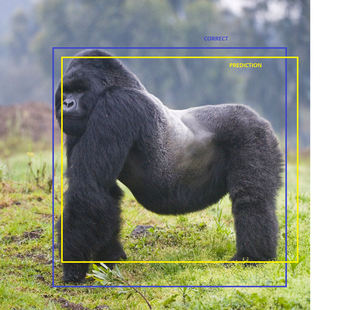
As shown in the example image above, the blue bounding box is the correct detection (label) and the yellow bounding box is the prediction, what the model is predicting. Note that the yellow box could also be something that a human would annotate as the object class.
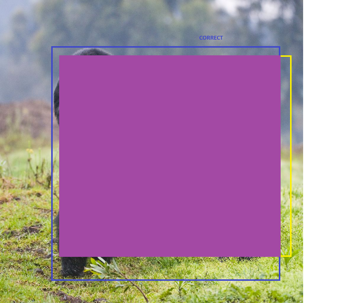
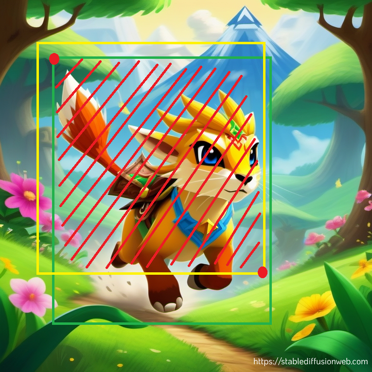
In this particular example, the Intersection is the area that is intersected, in common, between the two boxes, below marked in purple.
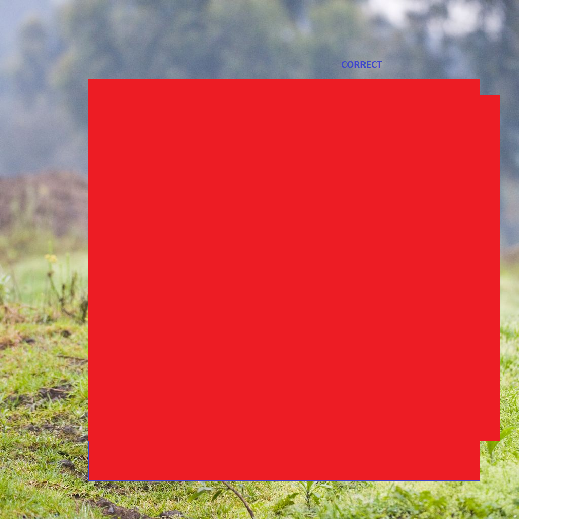
The Union, as it can be deduced from the word, it is the area combined of the two bounding boxes.
Mathematically speaking, the IoU formula is just the Intersection divided by Union. The result will be a value between 0 and 1. Value of 0 means the two boxes do not intersect at all and a value of 1 that they are identical (rare if not impossible). The higher the number the more accurate the prediction by the model, or annotation done by a human, is. When talking about IoU, values over 0.5 are considered as “almost acceptable”, over 0.7 “good” and over 0.9 “great”.
How to calculate Intersection and Union areas
Let’s take as example this image (created with Stable Diffusion) with the correct bounding box (Green) and the prediction (Yellow):
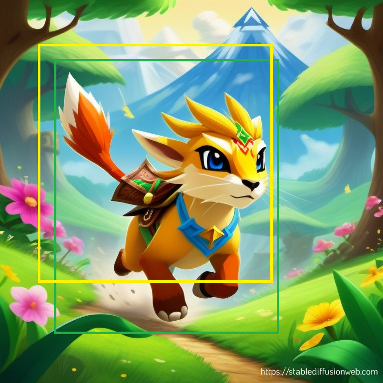
In computer vision the origin of the coordinates starts from left top corner. This means that if were to add coordinates to this image, we would have X = 0 and Y = 0 on the left top corner of the image, and X = 768 and Y = 768 at the bottom right corner (the image is 768 by 768 pixels), like this:
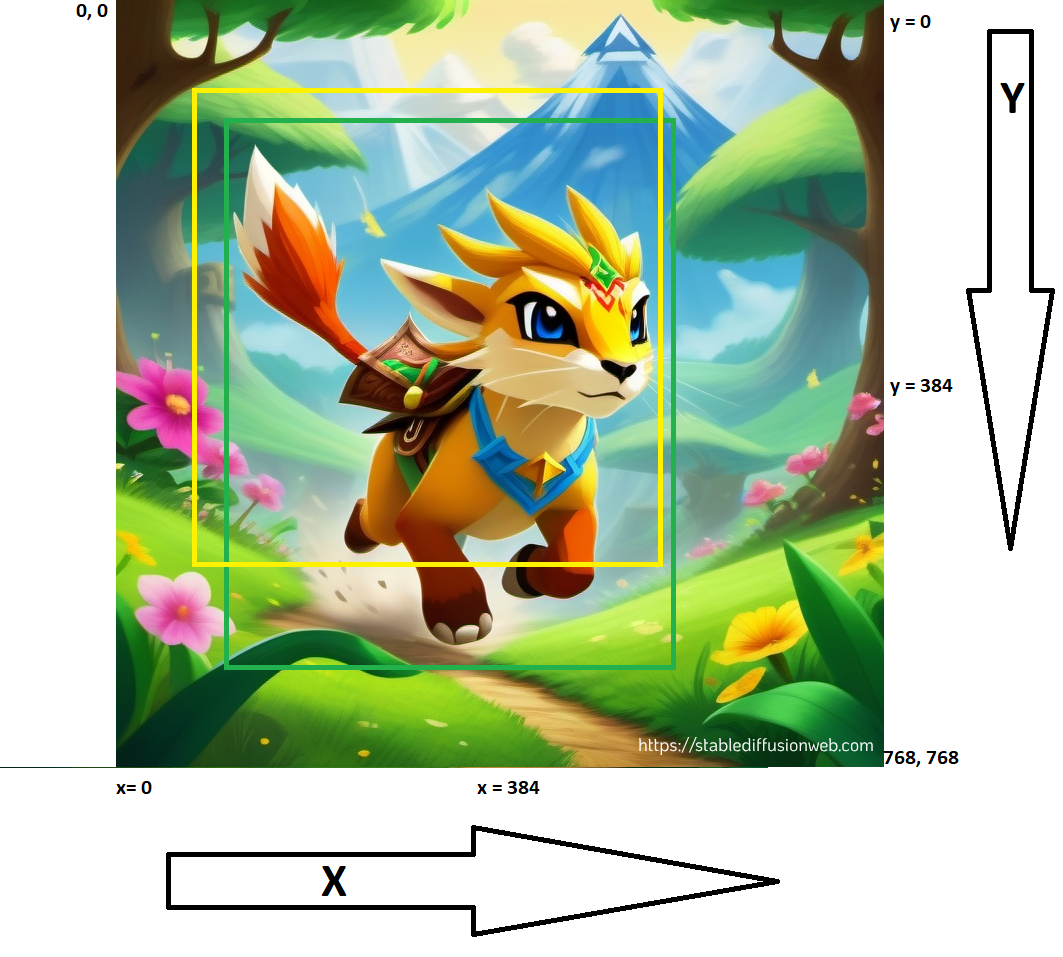
X grows from left to right and Y grows from top to bottom in this plane.
Now keeping this in mind, we want to calculate the area of intersection in this image. Having just the top left corner and the bottom right corner will suffice. If you work with YOLO for example you will need a bit different approach, more on it later. In our case then these coordinates would be the green top left corner (Label) and the yellow bottom right corner (prediction), like so:
The way we can calculate these coordinates is pretty straight forward.
For X of the left top corner for the intersection, we will take the MAX X coordinate of the top left corner of each bounding boxes. For Y of the left top corner for the intersection, we will do exactly the same, MAX Y coordinate of the top left corner each bounding boxes.
By looking at the image and the red dot, it is clear that the left top corner of the intersection will be then the X,Y left corner of the green bbox.
For the X of the bottom right corner for the intersection, we will instead take the MIN X coordinate of the bottom right corner of each bounding boxes. For the Y of the bottom right corner for the intesection, we will take the MIN Y coordinate f the bottom right corner of each bounding boxes.
In this case, it will be the yellow bottom right corner.
Note that that in this particulare case we are getting a pair X,Y from the same origin, same box, but this is not always the case. Example:
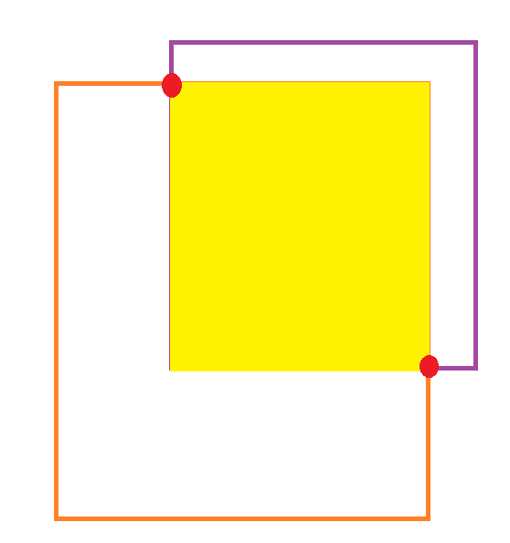
By looking at the image, to take the coordinates of the yellow area (intersection) the top left corner will be
X1, Y1 = PurpleX, OrangeY
Remember we take the MAX of the X and Y
X2, Y2 = OrangeX, PurpleY.
Hopefully this concept is clear at this point.
The Union area is simply just summing up both bounding boxes (taken into consideration to remove the union, else you add it twice).
Let’s do a code implementation of the IoU:
import numpy as np

def calculate_iou(predictions: np.ndarray,
        labels: np.ndarray,
        format: str = "x1y1x2y2") -> float:
    """
    Calculates IoU for x1y1x2y2 or xywh bounding boxes

    Parameters:
        predictions (numpy.ndarray): Predictions done by model
        labels (numpy.ndarray): Ground truth
        format (str): x1y1x2y2 format by default, xywh (YOLO style)

    Returns:
        float: Intersection over union
    """

    if format == "x1y1x2y2":
        box1_x1 = predictions[:, 0:1]
        box1_y1 = predictions[:, 1:2]
        box1_x2 = predictions[:, 2:3]
        box1_y2 = predictions[:, 3:4]
        box2_x1 = labels[:, 0:1]
        box2_y1 = labels[:, 1:2]
        box2_x2 = labels[:, 2:3]
        box2_y2 = labels[:, 3:4]

    elif format == "xywh":
        box1_x1 = predictions[:, 0:1] - predictions[:, 2:3] / 2
        box1_y1 = predictions[:, 1:2] - predictions[:, 3:4] / 2
        box1_x2 = predictions[:, 0:1] + predictions[:, 2:3] / 2
        box1_y2 = predictions[:, 1:2] + predictions[:, 3:4] / 2
        box2_x1 = labels[:, 0:1] - labels[:, 2:3] / 2
        box2_y1 = labels[:, 1:2] - labels[:, 3:4] / 2
        box2_x2 = labels[:, 0:1] + labels[:, 2:3] / 2
        box2_y2 = labels[:, 1:2] + labels[:, 3:4] / 2

    x1 = np.maximum(box1_x1, box2_x1)
    y1 = np.maximum(box1_y1, box2_y1)
    x2 = np.minimum(box1_x2, box2_x2)
    y2 = np.minimum(box1_y2, box2_y2)

    #clip(0) for when boxes do not intersect
    intersection = np.clip((x2 - x1), 0, None) * np.clip((y2 - y1), 0, None)
    box1_area = np.abs((box1_x2 - box1_x1) * (box1_y2 - box1_y1))
    box2_area = np.abs((box2_x2 - box2_x1) * (box2_y2 - box2_y1))

    iou = intersection / (box1_area + box2_area - intersection + 1e-6)
    return round(iou.item(), 2)


def test_intersection_over_union():
    # Test case 1: Two identical boxes, should result in IOU of 1.0
    box1 = np.array([2, 2, 4, 4])  # Format: [x1, y1, x2, y2]
    box2 = np.array([2, 2, 4, 4])
    iou = calculate_iou(np.array([box1]), np.array([box2]), format="x1y1x2y2")
    assert np.allclose(iou, 1.0), f"Test case 1 failed: {iou}"

    # Test case 2: Two non-overlapping boxes, should result in IOU of 0.0
    box3 = np.array([5, 5, 6, 6])
    iou = calculate_iou(np.array([box1]), np.array([box3]), format="x1y1x2y2")
    assert np.allclose(iou, 0.0), f"Test case 2 failed: {iou}"

    # Test case 3: Two partially overlapping boxes, should result in a valid IOU value
    box4 = np.array([3, 3, 5, 5])
    iou = calculate_iou(np.array([box1]), np.array([box4]), format="x1y1x2y2")
    assert 0.0 <= iou <= 1.0, f"Test case 3 failed: {iou}"

    # Test case 4: Test midpoint format with non-overlapping boxes
    box5_midpoint = np.array([3, 3, 2, 2])  # Format: [x_center, y_center, width, height]
    box6_midpoint = np.array([7, 7, 2, 2])
    iou = calculate_iou(np.array([box5_midpoint]), np.array([box6_midpoint]), format="xywh")
    assert np.allclose(iou, 0.0), f"Test case 4 failed: {iou}"

    print("All test cases passed!")

test_intersection_over_union()
OUTPUT: All test cases passed!
In the code above we first defined the function to calculate IoU as described earlier. In the function however we check the format of the boxes passed in input. As explained, we were discussing about x1y1 (top left) and x2y2 bottom right as coordinates, but there are knonwn systems like the one used in YOLO, where the coordinates of a box are given by x center, y center, height and width. For these cases we would need to convert the coordinates to that format, as it happens in the function.
When calculating the intersection, we also need to consider edge cases when there is no intersection at all, hence the clipping to 0.
Lastly, the IoU is calculated by dividing the intersection with the union (sum of the boxes areas minus intersection to not have it twice). The + 1e-6 term added to the denominator in the intersection over union (IoU) calculation is used to prevent division by zero. It is a small epsilon value added to the denominator to ensure numerical stability. This is commonly referred to as “smoothing” or “epsilon smoothing.”
A function for testing the IoU is then invoked to verify that the IoU calculation is working as expected. Testing your code is probably one of the best thing you can do. Creating test cases is time consuming, but nowadays with ChatGPT and other LLMs you can do this in a blink of an eye.
Non Max Suppression
Non Max Suppression is a technique to clean up the detections done by a model when doing object detection. Since we have understood now what is IoU, the Non Max Suppression is related to it. So first of all, what do mean by cleaning up the detections?
NMS is the technique of removing the less accurate bounding boxes and keep only 1 for that detection/class.
Each bounding box will have a confidence level (how confident the model is for that detection) between 0 and 1, example:
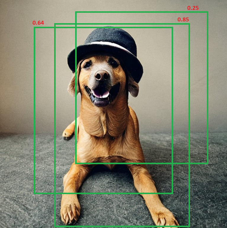
So how does this work in practice?
- First of all we select the BB with the highest confidence level. In this example the one with 0.85 score.
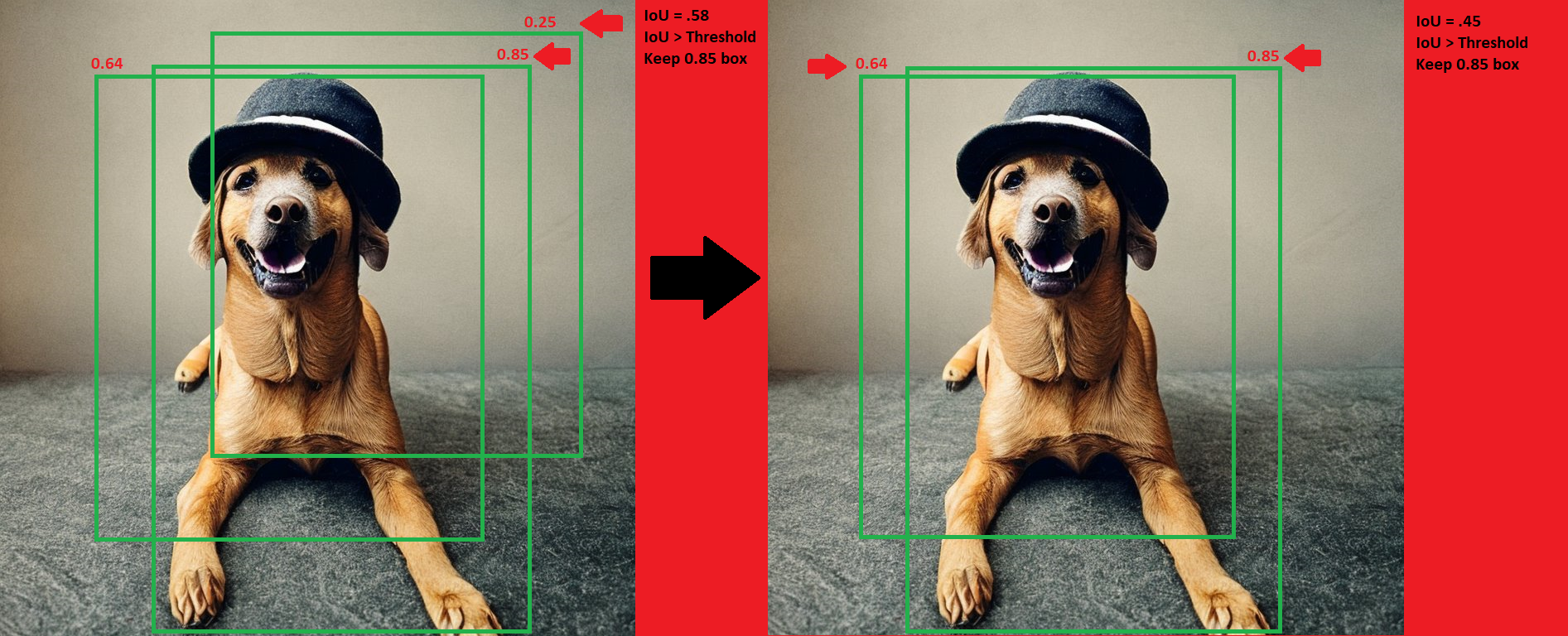
- For the NMS we need to set a hyperparameter that will be used to compare this IoU. For our example let’s select 0.4.
- Then we compare this BB to each individual other BB, and calculate the IoU as done above.
- If the IoU is greater than the hyperparameter, then we discard the second box. Step 3 and 4 and repeated until there is only 1 box remaining.
These steps they need to be done per class/detection. If in an image you have 3 objects, 3 different classes, you will not compare class 1 to class 2 boxes.
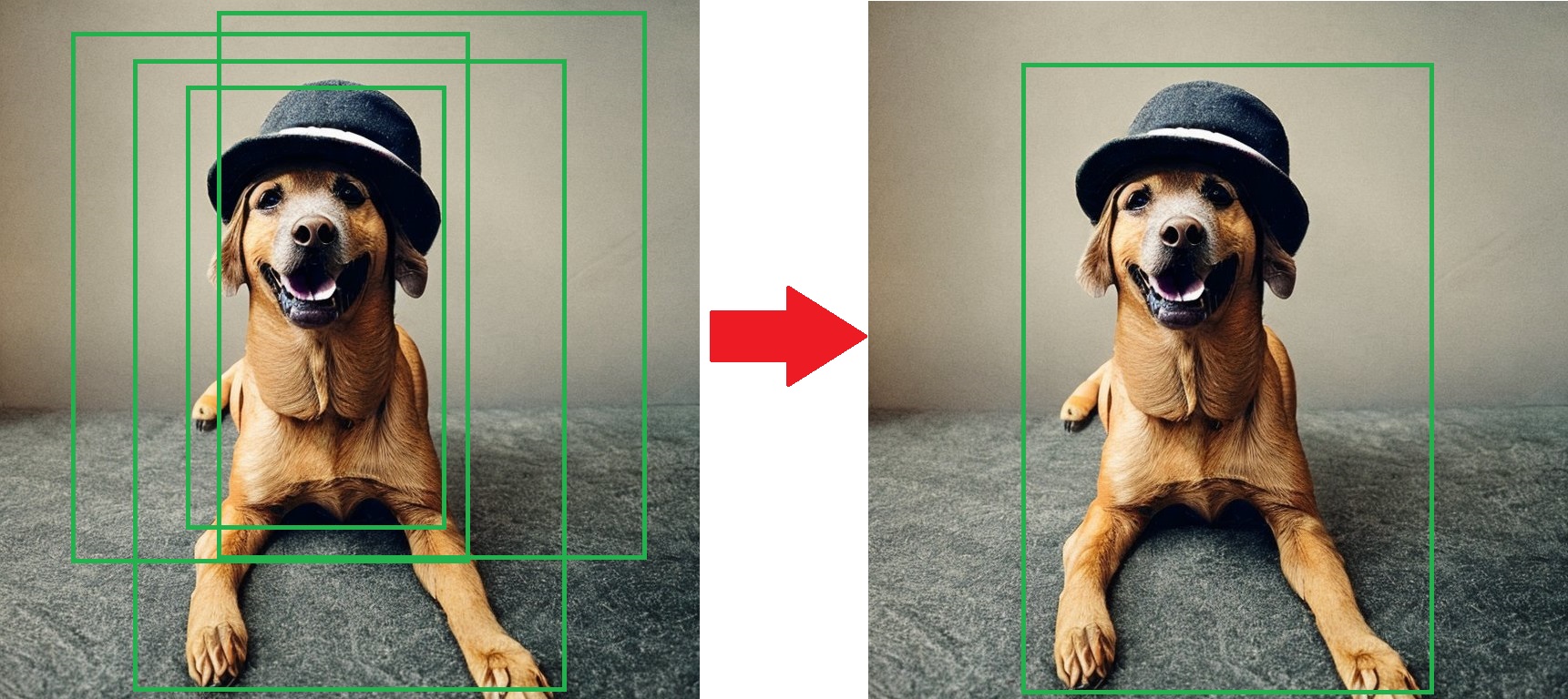
Let’s visualize this for an easier understanding:
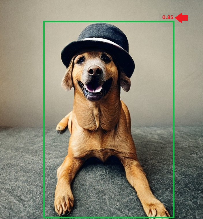
End Result
The concept is very simple, so let’s do a code implementation of this:
def non_max_suppressions(bboxes: List[np.array],
                        iou_threshold: int,
                        threshold: int) -> List[np.array]:
    """
    Non Max Suppression on a list of boxes

    Parameters:
        bboxes (numpy.ndarray): 2D array containing all bboxes. A box is predicted classe, probability score, x1y1x2y2
        iou_threshold (float): threshold used to select which box to keep
        threshold (float): min threshold to ignore predictions

    Returns:
        List[np.array]: Clean list of boxes
    """

    assert isinstance(bboxes, np.ndarray)

    bboxes = [box for box in bboxes if box[1] > threshold]
    bboxes = sorted(bboxes, key=lambda x: x[1], reverse=True)
    bboxes_after_nms = []

    while bboxes:
        chosen_box = bboxes.pop(0)

        bboxes = [
                    box for box in bboxes
                    if (box[0] != chosen_box[0] or calculate_iou(np.array([chosen_box[2:]]),np.array([box[2:]]))> iou_threshold)
                ]

        bboxes_after_nms.append(chosen_box)

    return bboxes_after_nms

# Test Case 1: Basic test case with no suppression
def test_nms_no_suppression():
    bboxes = np.array([
        [0, 0.8, 10, 10, 20, 20],
        [1, 0.7, 15, 15, 25, 25],
        [2, 0.6, 30, 30, 40, 40]
    ])
    iou_threshold = 0.5
    threshold = 0.5
    result = nms(bboxes, iou_threshold, threshold)
    assert np.allclose(result, bboxes)

# Test Case 2: Test with IoU-based suppression
def test_nms_with_suppression():
    bboxes = np.array([
        [0, 0.9, 10, 10, 20, 20],
        [0, 0.8, 15, 15, 25, 25],  # Suppressed due to IoU with previous box
        [1, 0.7, 20, 20, 30, 30],  # Not suppressed due to different class
        [2, 0.6, 35, 35, 45, 45]
    ])
    iou_threshold = 0.5
    threshold = 0.5
    result = nms(bboxes, iou_threshold, threshold)
    expected_result = np.array([
        [0, 0.9, 10, 10, 20, 20],
        [1, 0.7, 20, 20, 30, 30],
        [2, 0.6, 35, 35, 45, 45]
    ])
    assert np.allclose(result, expected_result)


# Run the test cases
test_nms_no_suppression()
test_nms_with_suppression()

print("All test cases passed!")
OUTPUT: All test cases passed!
HSV vs RGB vs GrayScale (Binary)
As final topic to conclude this blog post, I wanted to briefly discuss about RGB which probably most of the people have heard of and HSV, less likely and maybe Grey Scale even less.
All three are different color representations used in CV and image processing, and each has its own advantages for different tasks.
RGB (Red, Green, Blue)
RGB represents colors as combinations of red, green, and blue channels. Each pixel in an RGB image is described by three values, typically ranging from 0 to 255 for each channel, indicating the intensity of red, green, and blue light. Whenever you see an RGB image, you can think of it as an image made of 3 layers. Example:
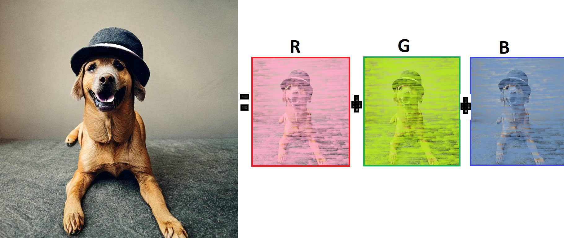
RGB is a widely used color model for displaying and capturing images. It is a straightforward representation of color and closely aligns with how our eyes perceive color, making it suitable for tasks like image display, visualization, and basic image processing operations. You can imagine an image as a matrix with numbers, where each pixel is a pair of 3 numbers, 1 per channel. If you imagine a picture as a matrix, you can already see that you could do some basic CV task by just working at pixel level.
HSV (Hue, Saturation, Value)
HSV represents colors based on three components:
Hue: It represents the type of color (e.g., red, blue, yellow) and is represented as an angle around a color wheel, typically ranging from 0 to 360 degrees.
Saturation: It measures the intensity of the color and ranges from 0 (no color, grayscale) to 100% (full color).
Value (Brightness): It represents the brightness of the color and ranges from 0 (black) to 100% (full brightness).
HSV is particularly useful for tasks that involve color segmentation, object tracking, and image processing operations where you want to isolate or manipulate specific colors. It separates the color information from brightness, making it more robust to changes in lighting conditions.
Binary (Grayscale)
Binary or grayscale images represent colors using shades of gray. In a grayscale image, each pixel has a single value representing its brightness, ranging from 0 (black) to 255 (white) in an 8-bit grayscale image.
When to use each color model?
RGB is preferred when you need to display or work with images in their original color form, perform basic image operations like resizing, cropping, or when color information is not a primary consideration in the task (e.g., edge detection, simple object detection).
HSV instead is a better solution when your computer vision task requires distinguishing objects based on their color, or when you need to perform color-based segmentation, tracking, or any operation where color plays a crucial role in the analysis. HSV is less sensitive to changes in lighting conditions compared to RGB, which makes it more suitable for these tasks.
Grayscale images are used when color information is not needed or when simplifying an image for certain types of analysis or processing.
Let’s make a simple example on this image:
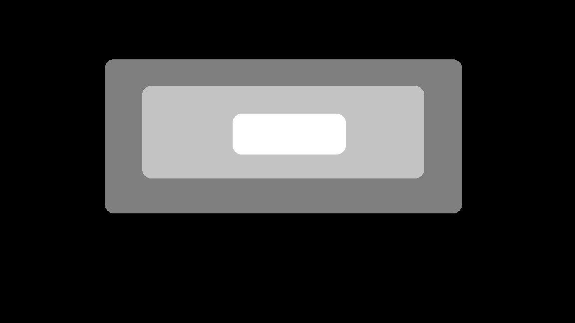
How can we detect the three different regions without doing anything complex? Which of the color scales would make more sense now?
Let’s try with Grayscale:
import cv2
from PIL import Image

image_path = ".\images\IOU\Mask.png"

img = cv2.imread(image_path)

for low_bound in [1, 150, 250]:

    gray = cv2.cvtColor(img, cv2.COLOR_BGR2GRAY)

    _, mask = cv2.threshold(gray, low_bound, 255, cv2.THRESH_BINARY)

    mask_to_image = Image.fromarray(mask).save(f"{low_bound}_mask.png")

    contours, _ = cv2.findContours(mask, cv2.RETR_EXTERNAL, cv2.CHAIN_APPROX_SIMPLE)
    result_img = img.copy()
    cv2.imwrite(f"{low_bound}_contour.png", cv2.drawContours(result_img, contours, -1, (0, 255, 0), 2))
So what is going on in here?
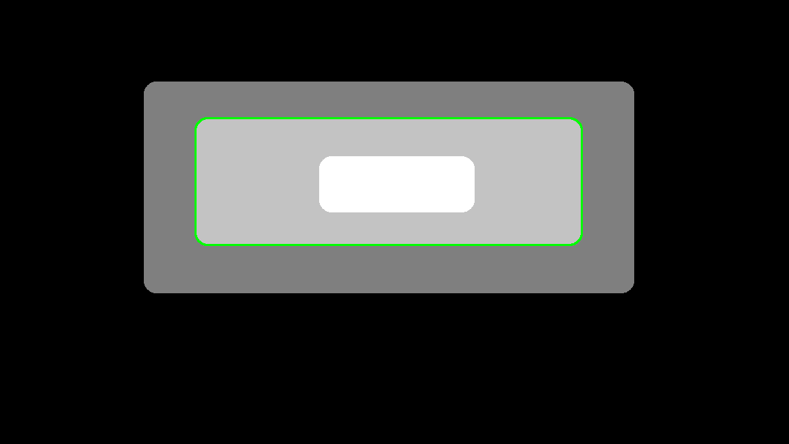
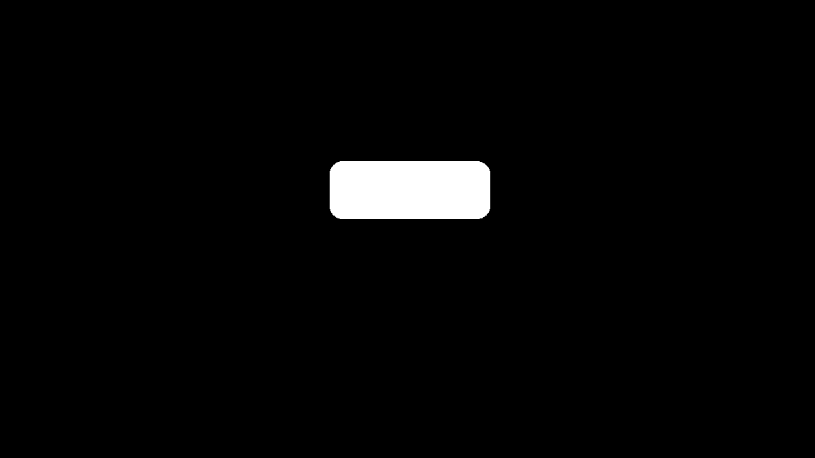
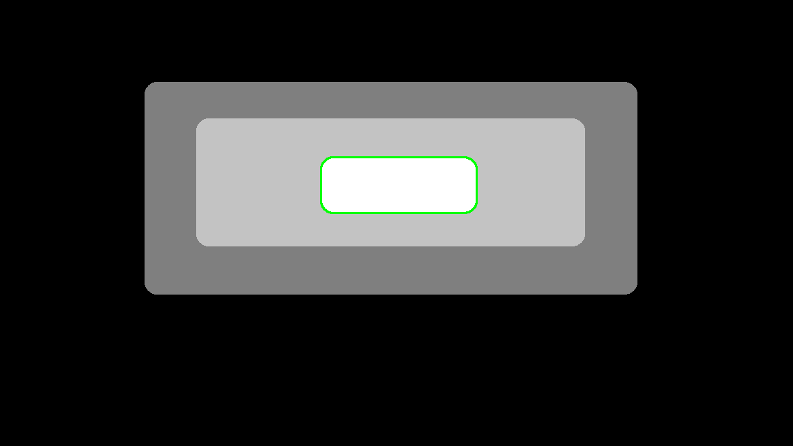
First we read the mask image with cv2. Then, we have a loop for binary values of 1, 150, 250. Now remember, the image had black as background, which has 0 value in the grayscale. So in this particulare case, to detect the biggest figure, a value of 1 will do. The medium size figure has surely a higher value, and after a trail and error, it looks like the value of 150 was high enough to detect that particular area. The inner figure is white (255 on a the grayscale) so 250 will be enough to detect it. Then for each detection we output the mask and the overlay on the original image by drawing the contours in green.
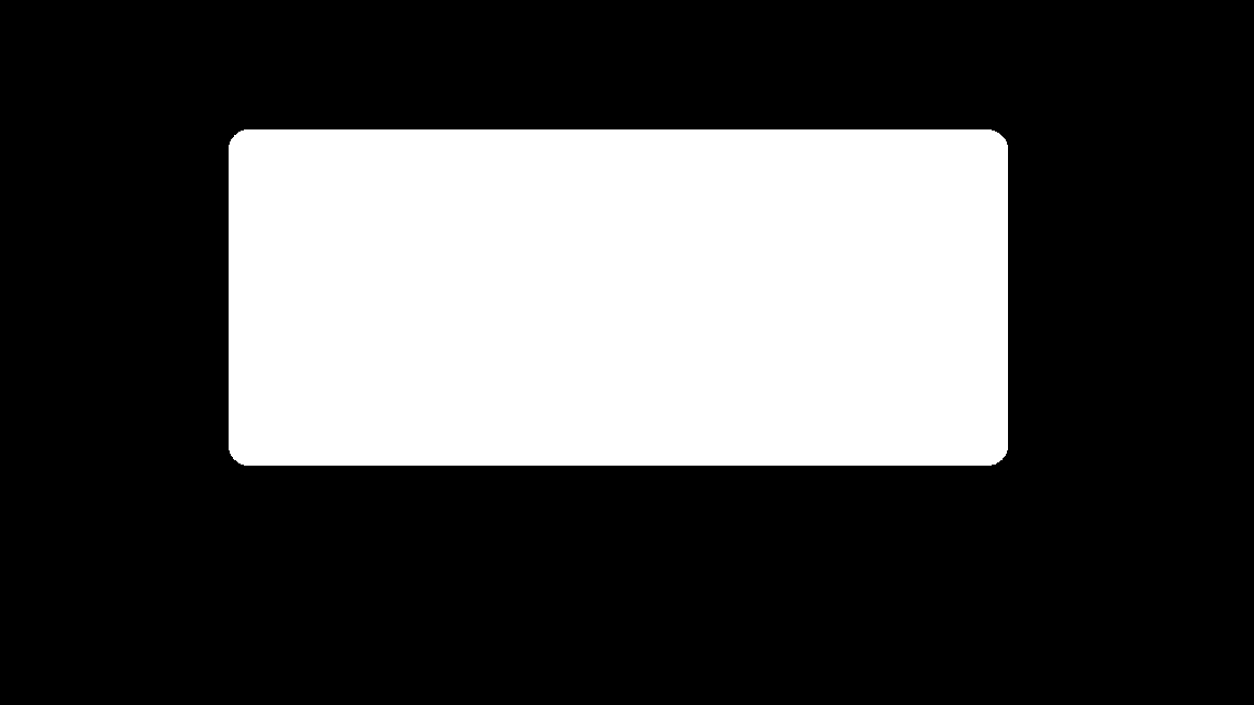
These are the outputs.
1 value MASK and Contour
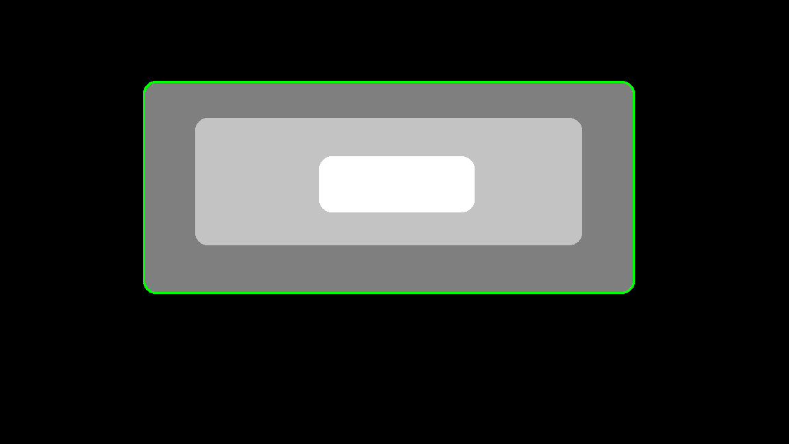
150 value MASK and Contour
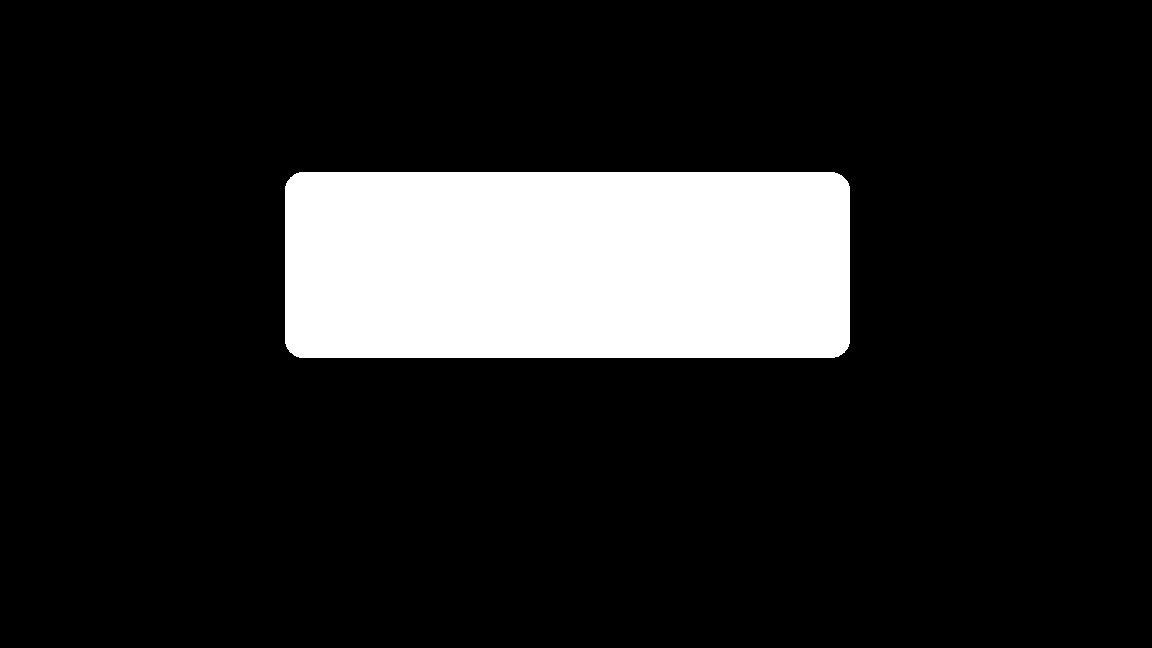
250 value MASK and Contour
Looks good!