Embeddings, Vector Databases, RAG, KNN, Hierarchical Navigable Small World (HNSW)
There is no doubt that the hype about LLMs is not going to stop anytime soon and whatever related to them, directly or indirectly, can be beneficial to learn about not to fall behind. One thing I have spent some time on lately is exploring more about Embeddings and related topics such as Vector Databases, especially after taking the free course on DeepLearning.AI about Vector DB with Weaviate. So first of all, what is an embedding?
What is an Embedding?
Simply put an embedding is a representation of an input that the machine/neural network can understand. Neural Networks work with numbers, so whether you are working with strings/texts/corpora, images or audio (by using the spectrogram for example), the input can be converted, translated into numbers.
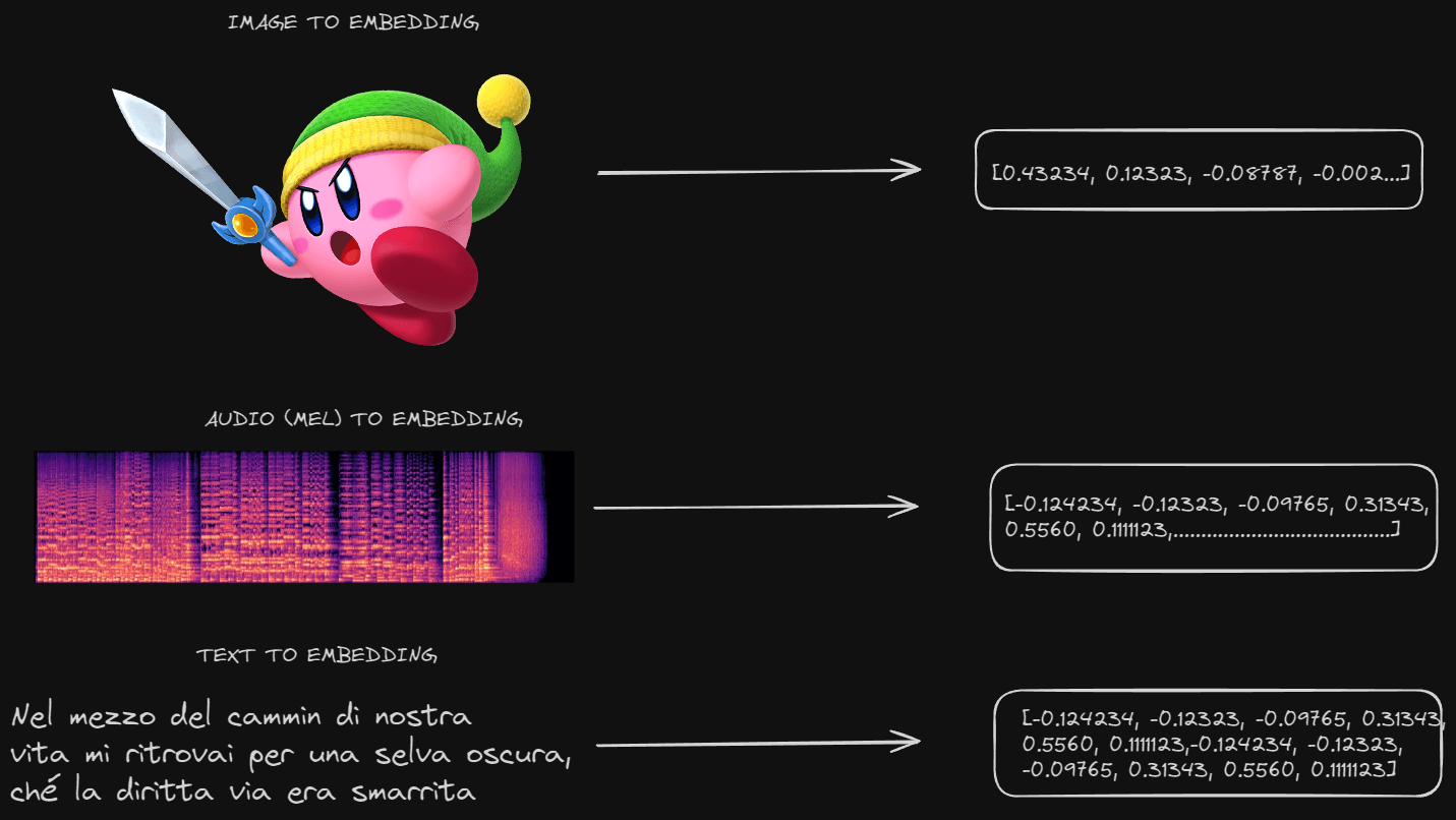
Vector Embeddings capture the meaning of the data and because of that, it is possible to perform semantic similarity and calculate how close different embeddings are between each other as points in vector spaces.
As an example, we can do an embeddings on a string with the SentenceTransformer from HuggingFace
from sentence_transformers import SentenceTransformer

model = SentenceTransformer('paraphrase-MiniLM-L6-v2')
encoded_string = model.encode("Nel mezzo del cammin di nostra vita mi ritrovai per una selva oscura, ché la diritta via era smarrita")

print(encoded_string)

[-3.15973699e-01  4.09273297e-01  6.94288164e-02 -1.96312413e-01
 -2.34583348e-01  2.93838233e-03  3.02226394e-01  2.28147089e-01
  3.36352050e-01  6.24060445e-02  6.64426565e-01 -5.60386181e-02
  6.29706532e-02  1.16161332e-01 -2.45653048e-01 -3.48773062e-01
  4.12333995e-01  8.48981798e-01  1.08630642e-01  2.32740670e-01
  6.35655820e-01 -2.11040955e-02 -1.27629459e-01 -1.44310623e-01
 -9.59611759e-02  3.05243492e-01 -1.07371323e-01 -4.92691845e-02
  1.45260200e-01 -2.01114304e-02  6.69209138e-02  4.91139263e-01
  2.26453960e-01  1.29266232e-01 -3.79163660e-02 -9.12928581e-03
 -2.69731104e-01 -3.12873155e-01 -1.93256903e-02  7.12252259e-01
 -3.78831774e-01 -8.95979032e-02 -2.58814037e-01  1.39955610e-01
  1.31800890e-01 -4.81816143e-01 -1.71137024e-02  1.26334220e-01
  3.41216922e-02  1.78940132e-01 -6.30956411e-01 -1.68935031e-01
 -7.27595985e-02  9.16724559e-03  1.05521999e-01 -7.38528520e-02
  2.39386141e-01  7.20317721e-01  4.91228461e-01  3.58403414e-01
  1.24995202e-01  4.10273224e-01 -5.44807851e-01 -2.47548953e-01
  2.50771344e-01 -3.90279651e-01 -4.31115389e-01 -2.86828876e-02
 -6.85104504e-02  3.23182374e-01  2.21761957e-01 -2.36219481e-01
 -1.54280096e-01  1.27513245e-01  3.04423273e-02 -3.60787176e-02
  1.08959591e-02  1.87333554e-01 -3.69372278e-01 -3.00745398e-01
  5.83267748e-01  3.14851463e-01 -4.72452700e-01 -1.01550668e-01
  1.68532982e-01  9.98338610e-02  2.03354675e-02  1.34621486e-01
  4.61549968e-01 -1.04218900e-01  2.22757816e-01  1.35493875e-01
  1.92801893e-01 -3.63590360e-01  3.00530434e-01 -1.41213849e-01
 -9.12229065e-03  4.58983272e-01  3.85241210e-01  1.72893584e-01
  2.25460231e-01 -2.92333961e-02 -2.29104459e-01  3.93774390e-01
 -2.98486263e-01 -9.71634313e-02  4.23806429e-01 -1.28027812e-01
  1.51418494e-02  4.96835649e-01 -6.03993349e-02  1.43707678e-01
 -5.64068496e-01 -3.13431114e-01  8.17491412e-02 -4.80100840e-01
  2.90427089e-01 -1.18213125e-01 -3.85904871e-02  9.62872878e-02
  1.38658091e-01 -3.30970407e-01 -3.04995418e-01 -8.89642388e-02
 -2.35730857e-01  1.02028750e-01  1.21251307e-01 -4.69212048e-03
 -1.86547816e-01  2.19465137e-01  1.36795565e-01  2.41343573e-01
 -2.02754084e-02 -1.38922006e-01 -2.83526838e-01  1.22377977e-01
  8.74637514e-02  1.92729570e-02 -4.24213141e-01  3.10779456e-03
 -7.19024301e-01 -4.36037838e-01  1.51090682e-01  2.82260448e-01
  2.72028387e-01 -3.83399606e-01  3.73818755e-01  1.88194960e-01
  2.48210534e-01 -3.49843234e-01  2.50031054e-02 -2.81302333e-01
  1.58814371e-01 -1.52342021e-01  1.55591980e-01 -5.39620221e-01
 -4.85759586e-01  4.93907571e-01  1.77475333e-01 -2.60481313e-02
  5.59068471e-02 -2.52387404e-01 -2.03820542e-02  1.65435523e-01
  2.29267299e-01 -1.62933266e-03 -4.35095251e-01  2.52411991e-01
 -2.88910210e-01  2.03594595e-01  2.52768606e-01  9.98502597e-02
 -2.74871476e-02  1.80527464e-01  4.01465327e-01  3.23309839e-01
  2.83275813e-01  4.54687290e-02 -2.39591971e-01 -2.07006633e-01
 -6.61132693e-01 -1.58638090e-01  3.64588108e-03  2.44528875e-01
 -1.26831099e-01  9.48398039e-02 -6.94694445e-02  3.23251300e-02
 -3.62637460e-01  1.38776571e-01 -1.16848268e-01 -5.35371676e-02
  2.06717700e-01  1.78061754e-01  1.72948137e-01  1.12204701e-01
  4.69952255e-01  8.75928029e-02 -3.59309137e-01 -1.43663704e-01
 -2.90623099e-01  5.37751243e-02  2.77311937e-03 -4.12063897e-01
  3.43293428e-01  1.69361085e-01 -2.53183842e-01  4.30487655e-02
 -3.46294820e-01  9.50148329e-02 -2.34710827e-01  1.96986109e-01
  5.48437834e-01  4.68549877e-01  3.76453668e-01  3.95353466e-01
 -7.89191574e-02  1.32808626e-01  1.94547623e-02  1.45085424e-01
  1.67537481e-01 -6.67654335e-01  9.22509655e-03  2.52136514e-02
  3.70544493e-02  1.20272532e-01 -9.06059816e-02  4.03778613e-01
 -2.24450529e-01 -1.14504710e-01 -4.56139624e-01 -1.78313971e-01
 -2.07843363e-01 -1.35141373e-01 -4.87709999e-01 -2.43196175e-01
  6.23809934e-01 -3.97263840e-02 -5.51651776e-01  2.43138254e-01
 -7.96630085e-02 -1.76247612e-01 -4.02588010e-01 -1.94599733e-01
 -5.86369991e-01 -7.41731077e-02  4.99878287e-01 -3.35904621e-02
 -1.25402555e-01  1.76211074e-01  2.53314704e-01  5.45195758e-01
 -4.91634786e-01  1.61703140e-01  5.24560213e-02 -3.59673232e-01
 -4.98636127e-01 -2.21637800e-01 -8.44015926e-02  3.00983578e-01
 ....]
Let’s now embed couple of sentences and visualize them to see how visually they look alike:
import seaborn as sns
import matplotlib.pyplot as plt

sentences = ["Leonardo da Vinci (1452–1519) was a Renaissance polymath renowned for his diverse talents and contributions to art, science, and innovation. Widely considered one of the greatest artists in history, he created masterpieces such as the Mona Lisa and The Last Supper.",
"Vinci's insatiable curiosity led him to make groundbreaking scientific observations and sketches in fields ranging from anatomy and engineering to astronomy, showcasing his remarkable intellect and leaving an indelible mark on both the arts and sciences.",
"Gorillas are herbivorous, predominantly ground-dwelling great apes that inhabit the tropical forests of equatorial Africa"]

embeddings = model.encode(sentences)

for i, embedding in enumerate(embeddings):
    sns.heatmap(embeddings[i].reshape(-1,384),cmap="Reds",center=0,square=False)
    plt.gcf().set_size_inches(24,1)
    plt.axis('off')
    plt.show()
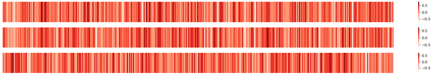
From the plot above you can kind of see that the two first sentences are having a somewhat similar representation than the third one
Measuring similarity/distance between embeddings
There are various ways to calculate distances/similarities between two vector embeddings, and the choice often depends on the specific characteristics of the data and the problem you are trying to solve. Let’s check some:
- Euclidean Distance:
- The Euclidean distance between two vectors A and B in an n-dimensional space is given by:
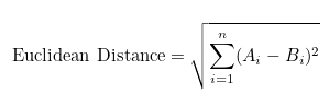
- It measures the straight-line distance between two points and the calculation goes as follows:
- For each dimension i, subtract the corresponding components A at i and B at i
- Square the result of each subtraction
- Sum up all the squared differences from i = 1 to i = n
- Calculate square root of the sum
This can be represented as this (for simplicity in a 2-D plane):
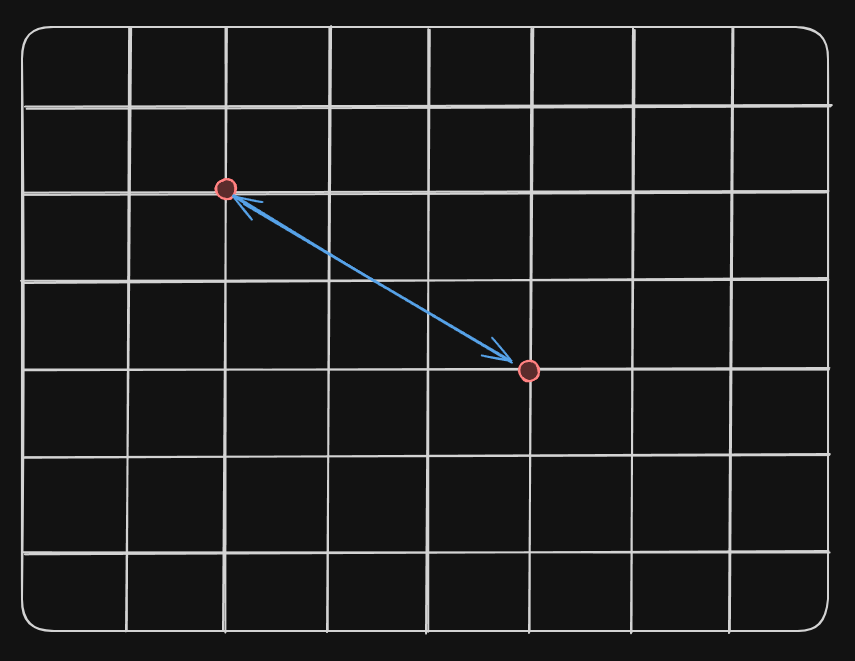
In Python you can implement it as this:
np.linalg.norm((emb_A - emb_B), ord=2) - Manhattan (L1) Distance
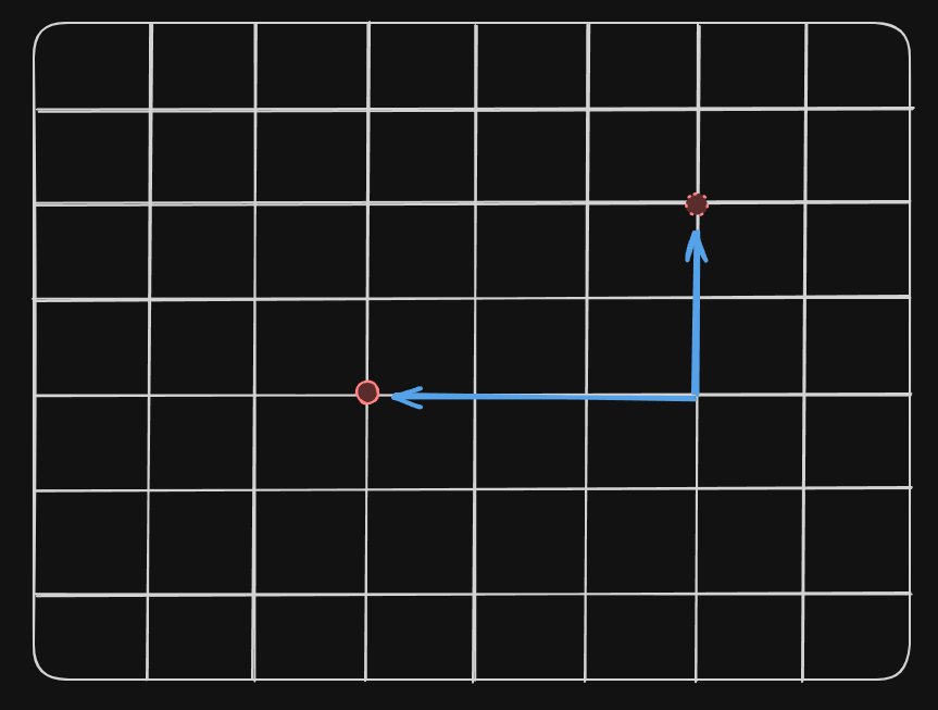
- The L1 Distance measures the distance between two points if it was only possible to move along one axis per time. You can imagine it as the distance along the grid lines of a rectangular grid, hence the name, from the layout of the streets in Manhattan.
- The distance is given by the sum of the absolute differences between their corresponding elements.
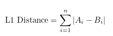
And it can be represented as this below:
In Python you can implement it as:
np.linalg.norm((emb_A - emb_B), ord=1) - Cosine Similarity or Dissimilarity (Distance)
- With Cosine Similarity it is measured the cosine of the angle between two vectors.
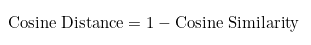
- Cosine Distance is just 1 - Cosine Similarity
- The range for Cosine Similarity is [-1, 1] where -1 is totally opposite vectors and +1 totally similar.
- The range for Cosine Distance is [0, 2], where 0 is identical vectors and 2 totally different.
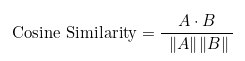
Where A⋅B is the dot product of the vectors A and B
Where ∥A∥ is the magnitude of the vector A, and ∥B∥ for the B vector.
The formula then is the dot product of the vectors divided by the product of their magnitude.
The cosine distance could be illustrated as follows:
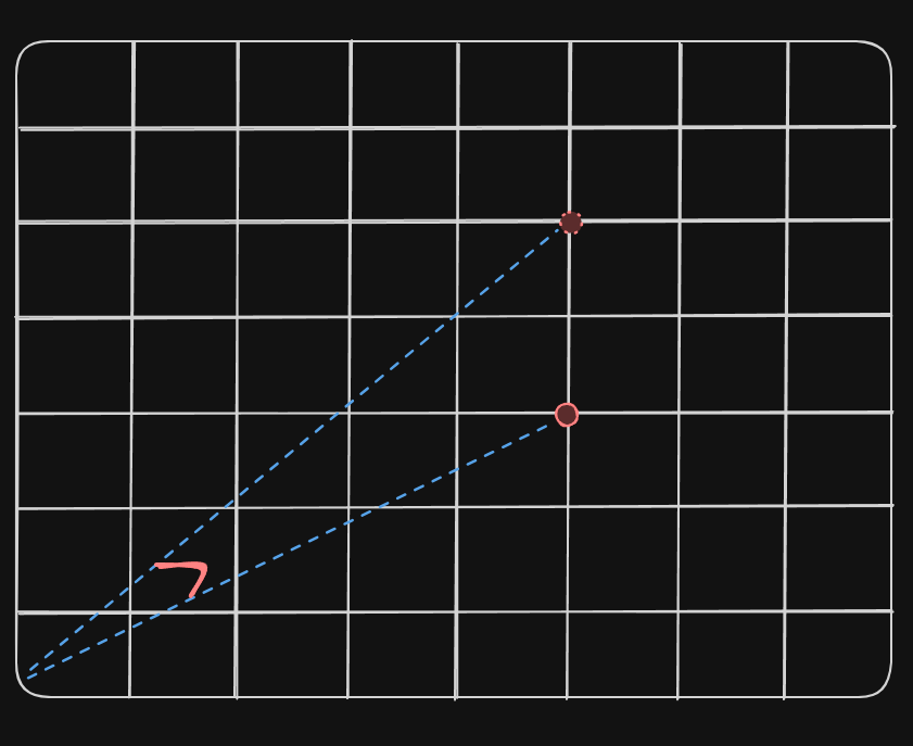
If we were to talk about embeddings for words/text, words with same meaning would point towards the same direction in space (this if we assume we represent the embeddings in a 2-D plane, X and Y).
In Python you can implement it like this:
cos_dis = 1 - np.dot(emb_A, emb_B) / (np.linalg.norm(emb_A) * np.linalg.norm(emb_B))
These are just some of the most common ways of calculating distances/similarities between vectors. There are many more but I selected those I have used personally at work as well.
Let’s test out if Cosine Similarity actually gives us the right feedback we are looking for. First we create some embeddings from some sentences and then compare them each to the rest.
import numpy as np
from sentence_transformers import SentenceTransformer
from itertools import combinations

model = SentenceTransformer('paraphrase-MiniLM-L6-v2')

sentences = ["Leonardo da Vinci (1452–1519) was a Renaissance polymath renowned for his diverse talents and contributions to art, science, and innovation. Widely considered one of the greatest artists in history, he created masterpieces such as the Mona Lisa and The Last Supper.",
"Vinci's insatiable curiosity led him to make groundbreaking scientific observations and sketches in fields ranging from anatomy and engineering to astronomy, showcasing his remarkable intellect and leaving an indelible mark on both the arts and sciences.",
"Gorillas are herbivorous, predominantly ground-dwelling great apes that inhabit the tropical forests of equatorial Africa"]


def cosine_similarity(vec1: np.ndarray, vec2: np.ndarray):
  cos_sim = (np.dot(vec1, vec2) / (np.linalg.norm(vec1) * np.linalg.norm(vec2)))
  return cos_sim

embeddings = model.encode(sentences)
permuted_pairs = combinations(embeddings, 2)

for pair in permuted_pairs:
    print(cosine_similarity(pair[0], pair[1]))
Output
0.5847281
-0.062435877
-0.06368498
The pairs combinations analysed are [[0, 1], [0, 2], [1, 2]] from the list. It is clear that when comparing the first sentence embedding against the third in the list OR the second to the third in the list, the values are negative, while when comparing the first to the second sentence, the cosine is positive and direction is towards 1.
Another example.
sentences = ["The enchanting display of colorful lights above the polar regions captivates onlookers, showcasing the splendid beauty of nature's cosmic ballet. The Northern Lights, or Aurora Borealis, mesmerize observers with their vibrant and ethereal dance in the night sky, a celestial phenomenon resulting from the interaction of charged particles with Earth's magnetic field.",
"The enchanting display of colorful lights above the polar regions captivates onlookers, showcasing the splendid beauty of nature's cosmic ballet."
             ]

embeddings = model.encode(sentences)
print(cosine_similarity(embeddings[0], embeddings[1]))
Output
0.8375309
The two sentences are of different length although both talk about the Aurora Borealis but with different words. Since the embeddings capture the meaning, we can see with the cosine similarity that the two are in fact close to each other.
RAG (Retrieval Augmented Generation)
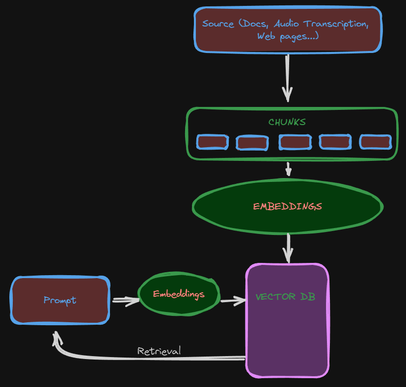
The acronym RAG is surely something we all have heard in the past months and there’s ton of material online available that explains how RAG works and all the techniques that can be used. At a basic level RAG allows you to retrieve information from a source based on a query/prompt you give. The source could be a series of documents, web pages, audio in the form of audio transcription etc. I actually had already created couple of implementations of this core idea of creating embeddings of a source and then query it:
- Langchain: https://ultragorira.github.io/2023/04/27/Langchain.html
- YouTube Querier: https://ultragorira.github.io/2023/06/08/YouTube_Querier_Langchain_and_Gradio.html
The idea is to chunk the data into smaller pieces, create embeddings of each chunk, store the embeddings in a VectorDB, which could be Chroma, FAIS, Weaviate etc. When prompting the LLM, the query is also embedded and then the search is done at embeddings level.
In a Vector DB there will be stored the embeddings that can be retrieved in a number of ways, cosine similarity or other metrics are used. Algorithmically, K-Nearest Neighbor (KNN) or variants of it are used.
K-NN
The most basic approach to go about K-NN is to comparing the query/prompt with all the embeddings found in the vector DB, sort by distance/similarity and take the top-K, where K could be 3 for example.
This approach is extremely slow and has a Big O Notation of O(n * d), where n is the num of embeddings and d is their dimensions. However, it is slow but very accurate.
Hierarchical Navigable Small World (HNSW)
In Similarity Search the metric that is mostly considered is Recall. A quicker although less precise method to retrieve embeddings is HNSW which is an algorithm for Approximate Nearest Neighbors (ANN). ANN is based on the idea of Six Degreees of Separation.
The concept of “Six Degrees of Separation” is a social theory that suggests that any two people in the world can be connected to each other through a chain of acquaintances with no more than six intermediaries. In other words, everyone is at most six steps away from any other person on Earth. The theory became popularized through a small-world experiment conducted by social psychologist Stanley Milgram in the 1960s. In Milgram’s experiment, participants were asked to send a letter to a target person (a specific individual chosen in the United States) through a chain of acquaintances. The participants were given the name and some background information about the target person and were instructed to send the letter to someone they knew who might be closer to the target. The chain continued until the letter reached the target person.
Milgram found that the average number of intermediaries in the chains was surprisingly small, typically around six. This led to the formulation of the idea that social networks are highly interconnected, and it takes only a few steps to connect any two people.
What is a NSW
NSW is a concept used in algorithms for approximate nearest neighbor search. The basic idea is to create a graph structure where each node is connected to its “navigable neighbors” in the high-dimensional space. This graph should exhibit the small-world property, meaning that nodes are well-connected, and it should be navigable, meaning that it allows for efficient exploration of the space. The algorithm aims to strike a balance between accuracy (finding neighbors that are close in the high-dimensional space) and efficiency (quickly navigating through the graph). Each nodes/vector can be connected to max 6 other vectors but this number can vary of course. The key is to achieve a small average shortest path length between nodes, allowing for quick exploration of the space while maintaining connectivity.
How does it work?
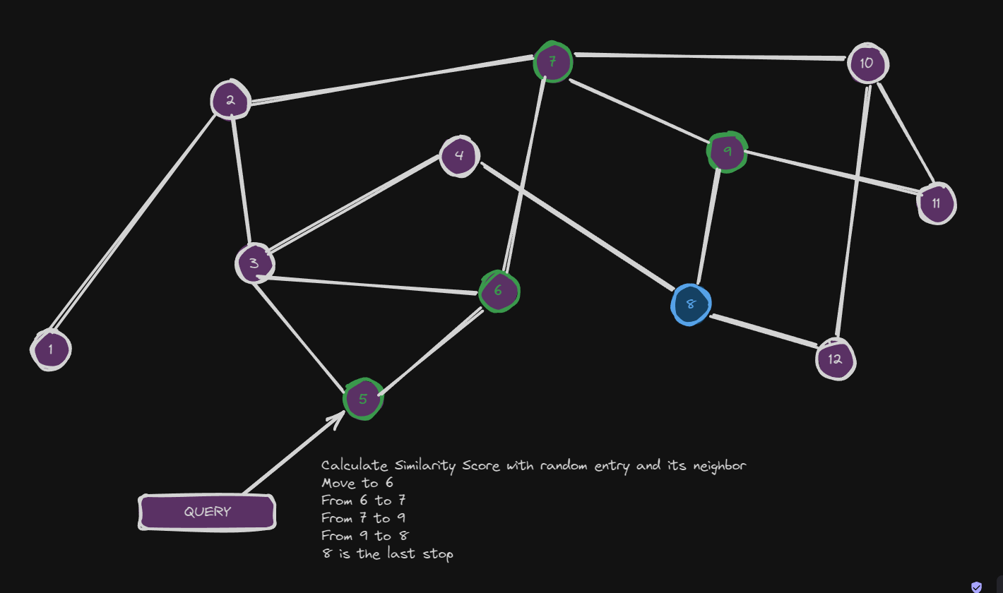
Let’s assume we have this sort of graph:
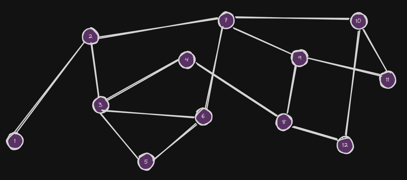
Each node in this graph is an embedding which could be for example chunk of a text but could be anything. For this case let’s assume they are chunked texts from some corpus.
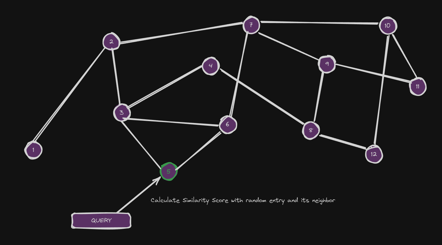
To find the top-k we initialize the embedded query at a random position and do the following:
- Compare the embedding of the Query to the Embedding of the randomly picked node, the comparison is calculate say the cosine similarity between the two.
- The same is done with the connected nodes to this randomly picked node and see if there is better results. If yes, move to that node. Repeat until the connected neighbor are having worse score.
- This process above is repeated from point 1 from different “entry points”
- The scores are sorted and kept only top-K
The HNSW makes use of Skip-List which is a data structure that allows for efficient search, insertion, and deletion of elements in a sorted sequence.
Node Structure:
Each element in the Skip List is represented by a node. Each node contains a key (or value) and a forward pointer that points to the next node in the same level.
Levels:
A Skip List consists of multiple levels. The bottom level contains all the elements in sorted order. Higher levels include fewer elements, and each element in a higher level has a forward pointer that skips over some elements in the lower levels.
Tower Structure:
Nodes with more than one level form towers. The top level of the Skip List contains a single tower that spans the entire sorted sequence.
The HNSW is basically a combination of NSW and Skip List.
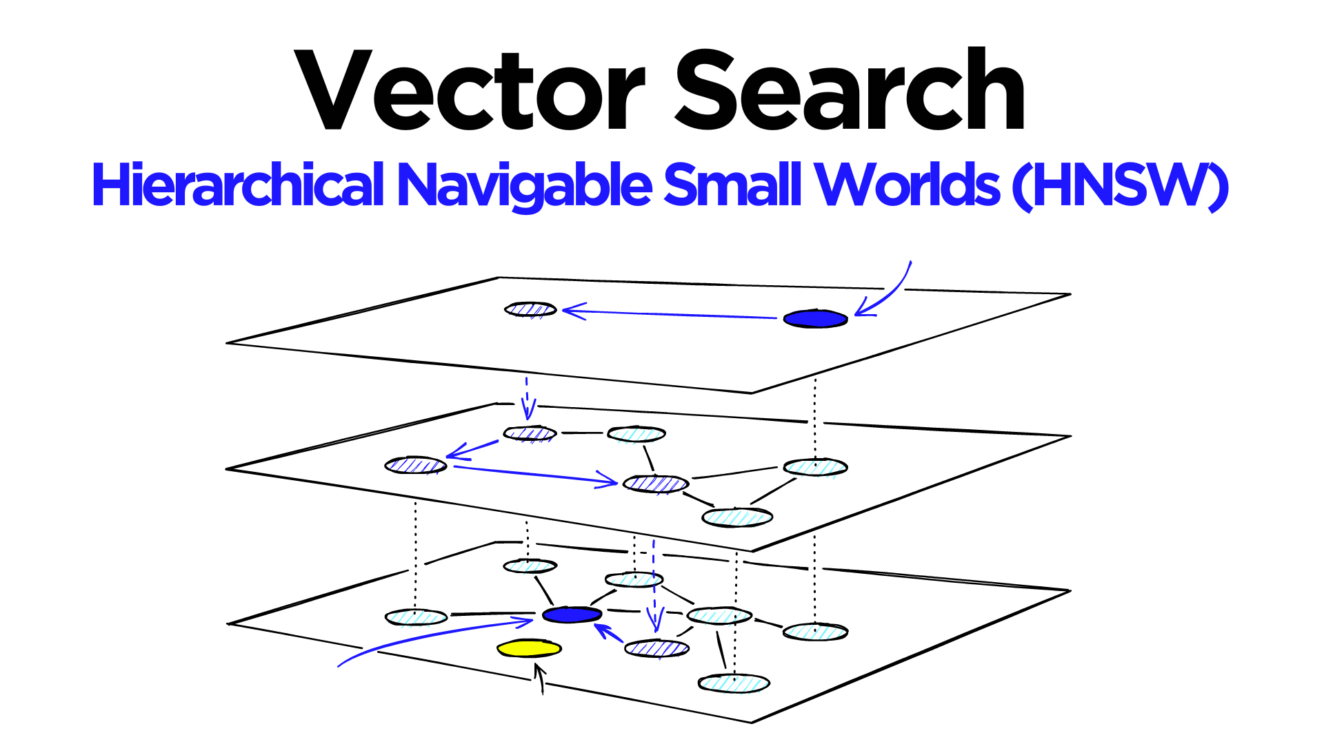 Photo taken from Pinecone: https://www.pinecone.io/learn/series/faiss/hnsw/
The lower level is the dense level where there are more nodes and connections. The top level is the sparse level.
How does it work?
As for the NSW, we have a random entry at the Sparse level (top one) and compare the similarity with its connections on the same level. Whichever has best score is selected and then we go to the lower level. The same similarity check is done at this level until we get the best one and then go lower. We stop until the local best is found.
This is again repeated with different entry.