Transformers - Attention is all you need
Image generated by Stable Diffusion. Prompt: “Transformer network artificial intelligence, 4k”
Neural Networks are the foundation of deep learning. You might have seen something like this below while reading about Deep Learning:
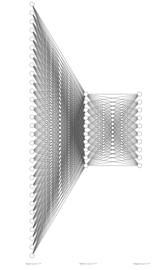
That’s a Multilayer Perceptron or MLP, one of the most basic Neural Network architectures, where you have an input layer, a hidden layer and an output layer. There are several different architectures nowadays but the one that changed the game is the Transformers architecture.
NLP and different architecture
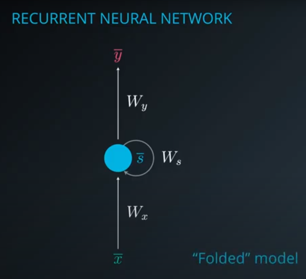
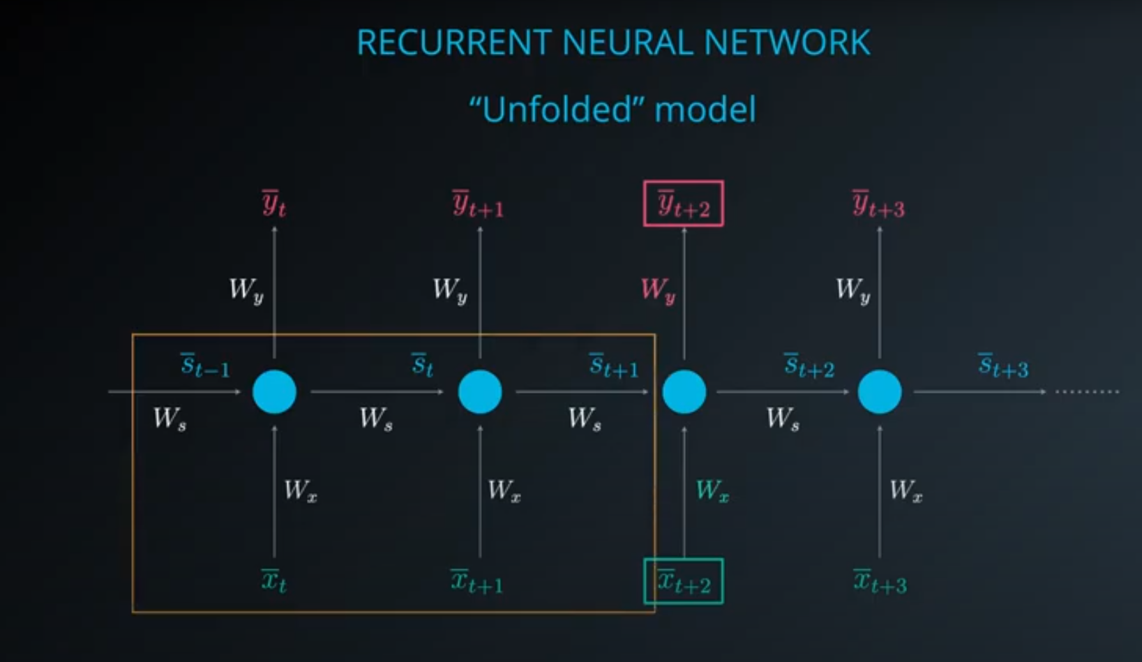
The usage of Transformers started from the NLP world where the data is a series of words. Before the advent of Transformers, the preferred architectures to deal with text data were Recurrent Neural Networks (RNNs). RNNs work with any sequence data, not just text.
Even though RNNs work with sequence data, they have some limitations such as:
- They do not work well with long sequences, and suffer of the so-called vanishing gradient. Basically when training the deep neural network, the gradients that are used to update the weights become so small or almost vanish when backpropagating to previous layers. RNNs cannot remember that much.
- They cannot be parallelized.
An alternative to RNNs is Long short-term memory neural network which is more complex and is able to handle longer series but due to the complexity of the network, they are slow to train.
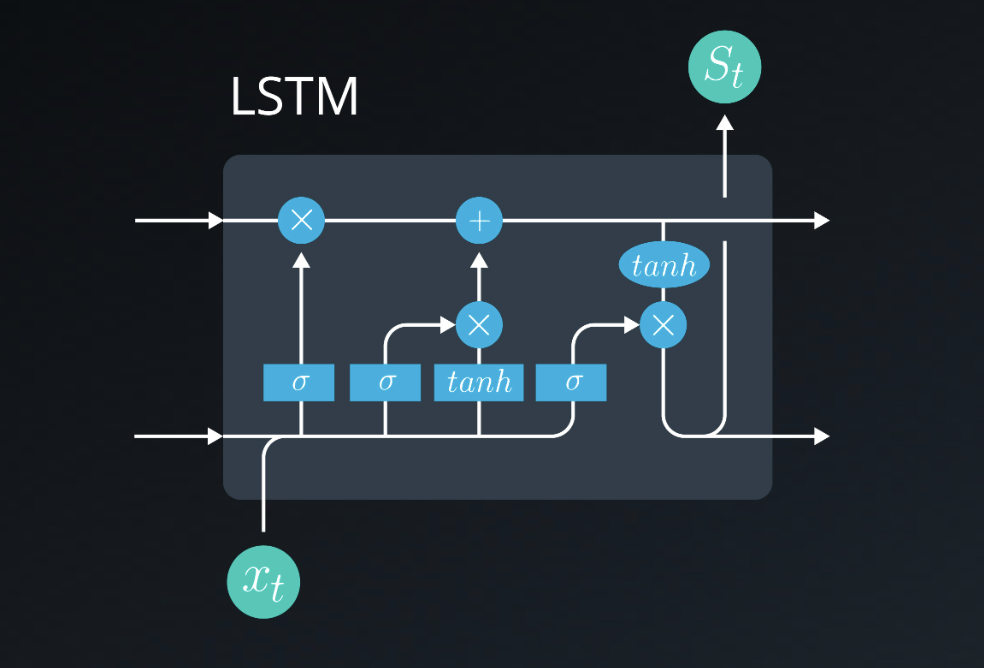
RNN and LSTM Images taken from the Deep Learning Nanodegree I completed from Udacity in 2022.
Transformers on the other hand shine with sequence data. The advantages of Transformers, compared to other networks are:
- They use the Attention mechanism which we will read more about later
- They are not recurrent and they can be parallelized
- They are faster to train
- Theoretically, given infinite amount of compute resources, they could handle infinite reference window (Just recently Claude by Anthropic was released with a 100k tokens, roughly 75k words per time.)
Attention mechanism
In 2017 a paper called Attention Is All You Need was published by Google. Back then the paper did not really catch much attention by the AI world and actually the authors of the paper would have never imagined that their work would have changed AI completely in a few years.
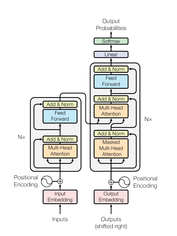
Transformers have an encoder (on the left) and decoder (on the right). The encoder’s job is to map the input sequence to a representation that includes all the information of the input. The same is then fed to the decoder and in steps generates an output. The previous output is also fed to the decoder.
Actually the encode is made of 6 encoders blocks, each one made up of a self-attention layer and a feed forward layer. The decoder is also made of 6 decoders, each of made of two self-attention layers and one feed forward layer.
Encoder
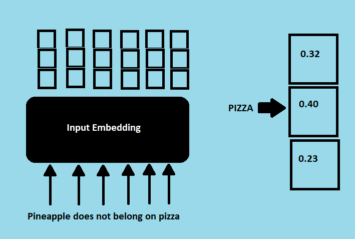
Firstly the sequence input, in this example a sentence but it could be any type of data (image, audio etc.), is fed into a word embedding layer which can be thought of something like a look-up table, where each word is represented as a vector. The word will be represented as a vector of numbers. The word embeddings are usually pre-trained using techniques like Word2Vec, GloVe, or FastText on large corpora to capture meaningful representations of words.
Next an information about the position of the input is added to the embeddings since the Transformers do not have the recurrence and do not know what is the position of the inputs due to their nature of parallelizing the inputs. This is done with Positional Encoding, by using sin and cos functions.
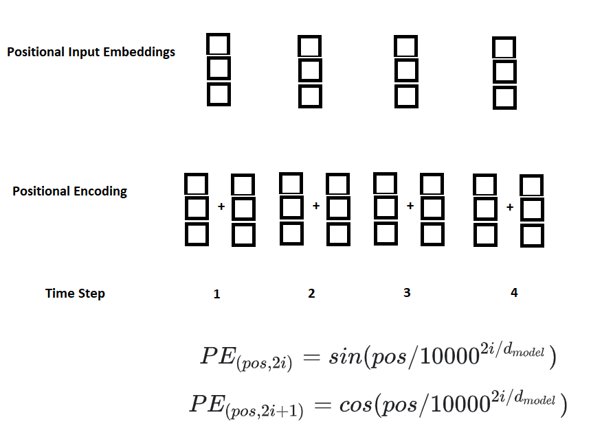
For odd timesteps the cos function is used, for even timesteps instead the sin function to calculate the vectors and add them to the embeddings vectors. Sine and Cosine are easy for the network to learn. These positional encodings or embeddings, are then added to the vector representation of the inputs.
Positional Encodings example:
import torch
import torch.nn as nn
import math
import matplotlib.pyplot as plt

class PositionalEncoding(nn.Module):
    def __init__(self, d_model, max_seq_len):
        super(PositionalEncoding, self).__init__()
        self.d_model = d_model

        # Create a matrix of shape (max_seq_len, d_model)
        pe = torch.zeros(max_seq_len, d_model)

        # Calculate the positional encodings
        position = torch.arange(0, max_seq_len, dtype=torch.float).unsqueeze(1)
        div_term = torch.exp(torch.arange(0, d_model, 2).float() * (-math.log(10000.0) / d_model))
        pe[:, 0::2] = torch.sin(position * div_term)
        pe[:, 1::2] = torch.cos(position * div_term)

        # Add a batch dimension to the positional encodings
        self.pe = pe.unsqueeze(0)

    def forward(self, x):
        # Add the positional encodings to the input tensor
        return x + self.pe[:, :x.size(1), :]

# Define the parameters
d_model = 512
max_seq_len = 100

# Create the positional encoding
pos_encoder = PositionalEncoding(d_model, max_seq_len)

# Generate the positional encodings for visualization
pos_encodings = pos_encoder.pe.squeeze(0).detach().numpy()

# Plot the positional encodings
plt.figure(figsize=(12, 6))
plt.imshow(pos_encodings, cmap='coolwarm', aspect='auto')
plt.xlabel('Embedding Dimension')
plt.ylabel('Position')
plt.colorbar(label='Value')
plt.title('Positional Encodings')
plt.show()
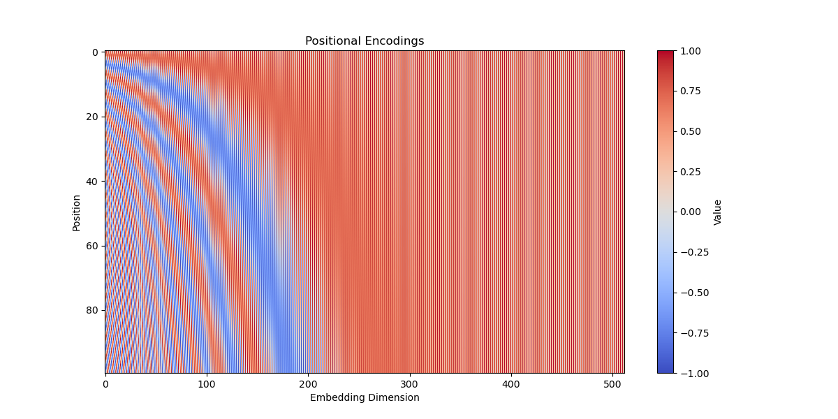
In this example there is a PositionalEncoding class that takes in the dimension of the model (d_model) and the maximum sequence length (max_seq_len) as arguments.
The matrix pe of shape (max_seq_len, d_model) holds the positional encodings. Positional encodings are calculated using the sine and cosine functions based on the position and the dimension of the model. These encodings are stored in the pe matrix.
In the forward method, positional encodings are added to the input tensor x. The positional encodings are sliced to match the length of the input sequence, and then added element-wise to the input tensor.
Encoder Layer
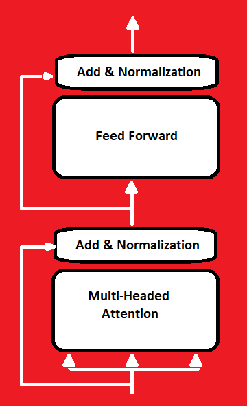
After the positional encodings are added to the input sequence, the main job of the encoder layer in a transformer model is to process the sequence and capture the contextual relationships between the tokens. The encoder layer consists of multiple sub-layers, typically including self-attention and feed-forward layers.
This block is constituted by Multi-Headed Attention followed by a fully connected network. Additionally there are also residual connections around both of Multi attention and fully connected network followed by a layer of normalization.
MULTI-HEADED ATTENTION
In the Multi-Headed Attention the so-called Self-Attention mechanism takes place. Self-attention is a mechanism that allows each position in the sequence to attend to other positions. It helps the model weigh the importance of different tokens within the sequence when encoding each token.
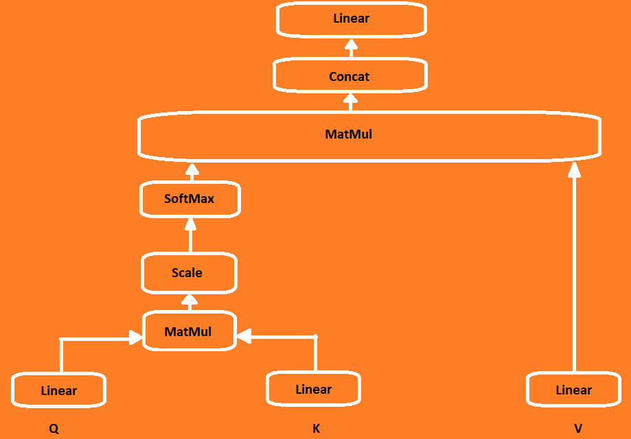
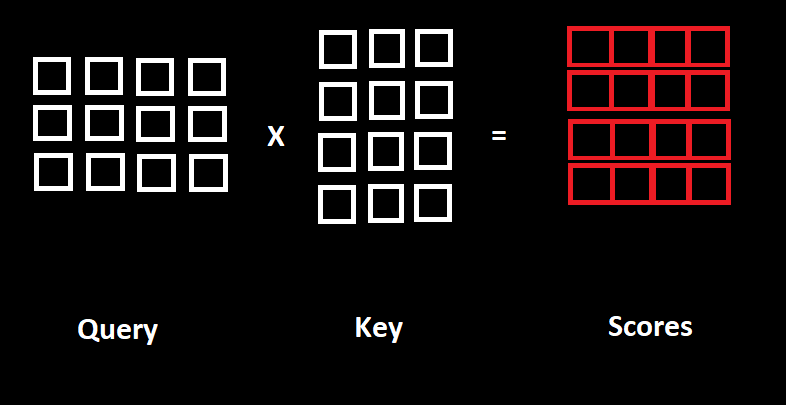
The inputs first are fed to three distinct fully connected layers to create the query (Q), key (K) and value (V) vectors. Here’s a good example of what query, key and value are.
A dot product is performed between Queries and Keys which produces a Scores matrix. The Scores matrix determines how much focus should each word be put into other words. The higher the score, the more focus.
Next the scores matrix are scaled down by the square root of the dimension of the queries and the keys. By scaling down the scores, the model can have more stable gradients during training, reducing the chances of exploding gradients that can hinder convergence.
Next a SoftMax is applied to get the attention weights which results in probabilities between 0 and 1. In this step, the Softmax normalizes the scores across the different positions in the sequence, emphasizing positions with higher scores and de-emphasizing positions with lower scores. Once obtained the attention weights, the same are multiplied with the Value matrix to get an output vector which is then fed into a Linear layer to process.
To make this a multi-headed attention process, it is achieved by splitting the Q, K, and V into additive vectors before self-attention is applied. This approach allows for multiple sets of attention weights to be computed, capturing different aspects of the input sequence. Each self-attention process is called head and each one produces an output vector that is concatenated by staking them together as a single vector. This concatenated vector preserves the information captured by each head and allows for further processing. This is then passed to a the last linear layer.
To recap: The use of multiple heads in the attention mechanism enables the model to learn diverse and contextually rich representations, as each head can focus on different aspects of the input sequence. The final concatenation and linear transformation before the last linear layer help to integrate the information from all the heads into a comprehensive representation for downstream tasks.
Next the output vector is added to the original input, called residual connection or skip connection. The purpose of this connection is to provide a direct path for the model to retain information from the original input, which helps in alleviating the vanishing gradient problem and improving the flow of gradients during training.
The output of this goes through Normalization layer. Layer normalization normalizes the activations across the feature dimension, ensuring that the inputs to the subsequent layers are centered and have a consistent scale. This normalization step helps in stabilizing the training process and improving the generalization of the model.
After normalization, the output is fed into a feed-forward network. The feed-forward network consists of linear layers with ReLU activation functions in between them. The purpose of this network is to apply non-linear transformations to the input, allowing the model to learn complex patterns and relationships in the data.
All the above is what an Encoder of a Transformer architecture is made of. Encoders can be stacked N times to be further encoded. Deeper architectures with more encoder layers can potentially capture more intricate patterns but might require more computational resources and longer training time.
Decoder Layer
The decoder has similar sub-layers as the encoder as it has two multi-headed attention layers, a feed-forward layer with residual connections and layer norm. Each multi-headed attention layer has a different job. The first multi-headed attention layer in the decoder, often called the masked self-attention layer, attends to the previous positions in the decoder’s input sequence, preventing any position from attending to subsequent positions. This masking ensures that during training, the model only has access to the previous tokens while predicting the next token, making it autoregressive.
The second multi-headed attention layer in the decoder is often referred to as the encoder-decoder attention layer. It attends to the encoder outputs, incorporating the attention information from the encoder into the decoder. This allows the decoder to focus on relevant parts of the input sequence while generating each output token.
As final portion, there is a linear layer and a softmax to get the probabilities. Let’s dive into a bit more on what happens in the Decoder.
The input goes through an embedding layer and positional encoding layer to get the positional embeddings. The positional embeddings are fed then to the first multi-headed attention layer which calculates the attention scores for the decoder’s input. In this multi-headed attention layer there is the so-called masked self-attention. How this works is that when computing attention scores, if you have a sentence like “I do not like pineapple on pizza”, when you are the word “pineapple”, you should not be able to see the words “on” and “pizza”. The current word should only have access to itself and previous words. To do this, a look-ahead mask is applied where the mask is added before calculating the soft-max and after scaling the scores. The mask has the same size of the attention scores matrix filled with 0s and -inf (negative infinity). When adding this mask to the scores you get the top right triangle filled with -inf. When applying softmax on this, the -inf become 0 effectively preventing the decoder from attending to future positions. This masking mechanism ensures that at each step of generation, the decoder can only focus on the relevant context from the past and the current position, mimicking the autoregressive behavior required for sequential generation tasks
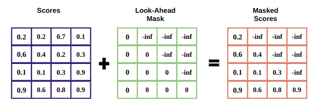
Image from https://ravikumarmn.github.io/concepts-you-should-know-before-getting-into/
The second multi-headed attention in the decoder, known as the encoder-decoder attention, serves a different purpose compared to the masked self-attention.
The input to the second multi-headed attention is typically a combination of the output from the first multi-headed attention layer in the decoder and the encoder outputs. This input allows the decoder to attend to the relevant information from the encoder while generating each output token.
Specifically, the output from the first multi-headed attention layer, which represents the decoder’s understanding of the input sequence so far, is used as the query (Q) for the encoder-decoder attention. The encoder outputs, which contain the encoded representation of the input sequence, serve as both the keys (K) and the values (V) for this attention mechanism.
The encoder-decoder attention mechanism enables the decoder to align itself with the relevant parts of the input sequence. By attending to the encoder outputs, the decoder can capture the context and information necessary for generating each output token based on the input sequence.
The output of the second multi-headed attention is then typically passed through a linear layer and further processed, usually involving residual connections, layer normalization, and feed-forward networks, similar to the sub-layers in the encoder and the first multi-headed attention layer in the decoder. These subsequent layers help refine the representations and transform them into suitable formats for generating the next output token.
The linear layer and softmax function at the end of the decoder serve the purpose of generating the probabilities over the vocabulary for each output token.
The output of the decoder after the last processing layers (such as residual connections, layer normalization, and feed-forward networks) is a vector representation of the context and information for generating the next output token. This vector typically has a dimensionality corresponding to the size of the vocabulary.
The linear layer is applied to this vector representation to transform it into a new vector with the same dimensionality as the vocabulary. The linear layer applies a linear transformation, typically implemented as a matrix multiplication, to map the representation to the desired output space.
The output of the linear layer is then passed through the softmax function, which converts the values in the vector into a probability distribution. The softmax function normalizes the values by exponentiating them and dividing by the sum of the exponentiated values. This normalization ensures that the output probabilities sum to 1.
The resulting probabilities represent the likelihood of each token in the vocabulary being the next output token. The decoder can then select the token with the highest probability as the predicted output. This process of selecting the token with the highest probability is often referred to as greedy decoding.
By applying the linear layer and softmax function at the end of the decoder, the model generates a probability distribution over the vocabulary, enabling it to make informed decisions about the most likely next token based on the given context and information from the input sequence.
The decoder continues generating tokens until it predicts an END token or until a predetermined maximum length is reached. The end token serves as a signal to stop the generation process and indicates the completion of the sequence.