CNN for Image Classification from scratch and with Transfer Learning
In this post I will walk you through on how to use Convolutional Neural Networks to build a model for image classification. I will first build the model from scratch and train it on a dataset. The second part of the post will do the implementation of the classifier by leveraging the so called transfer learning method.
The dataset
The dataset for this implementation is a subset of Google Landmarks V2. The data is divided into train and test sets but we will divide the train dataset in two, a train and a validation dataset. Generally you will always want to have 3 datasets when training a model: train, validation and test. The images are of landmarks around the world and the model will need to be able to identify what is the name of the landmark. There are a total of 50 different landmarks in this subset for a total of 3996 images in the test set, 1000 in the validation set and 1250 in the test set. The sizes of the pictures varies but we will normalize them to a fixed size of 224 by 224 pixels.
CNN Model from scratch
Let’s import the libraries
import torch
import numpy as np
import os
import requests, zipfile, io
from torchvision import transforms, models
from torchsampler import ImbalancedDatasetSampler
from torchvision import datasets
from torchsummary import summary
import torch.nn as nn
import torch.nn.functional as F
import torch.optim as optim
import splitfolders
from typing import Any
A few words on some of the libraries imported. ImbalancedDatasetSampler from torchsampler is a neat library that allows to rebalance class distributions when sampling. splitfolders I used to split the train dataset in train and validation, with a ratio of .8/.2. There are other ways of doing this but I found it very simple and straightforward and you can also split the data with a seed for reproducibility if you need to.
Download the data and split it
URL = 'https://udacity-dlnfd.s3-us-west-1.amazonaws.com/datasets/landmark_images.zip'
DATA_FOLDER = 'data'

if not(os.path.exists(DATA_FOLDER)):
    print(f"Downloading data to folder {DATA_FOLDER}")
    response = requests.get(URL)
    zipped_data = zipfile.ZipFile(io.BytesIO(response.content))
    zipped_data.extractall(DATA_FOLDER)
    print("Download complete and data extracted")
else:
    print(f"Data already download, check path {DATA_FOLDER}")

BATCH_SIZE = 32
NUM_WORKERS = 4
DATA_LOCATION = "data/landmark_images/"
SPLITS_RATIO = (.8, .2)
SEED = 1337

split = splitfolders.ratio(os.path.join(DATA_LOCATION, 'train'),
        output = os.path.join(DATA_LOCATION, 'split'),
        seed = SEED,
        ratio = SPLITS_RATIO,
        group_prefix=None
        )

train_dataset_path = os.path.join(DATA_LOCATION, 'split', 'train')
validation_dataset_path = os.path.join(DATA_LOCATION, 'split', 'val')
test_dataset_path = os.path.join(DATA_LOCATION, 'test')
Transform the data and DataLoaders Creation
We need to be able to load the images just downloaded as Tensors and feed them to our model. As you probably know already, neural networks whether we are talking about strings, images, video etc. the input needs to be converted to a Tensor, to numbers. For our model we will have a two different “transformation”, one for the train dataset and one for both the validation and test dataset. For the test dataset we will resize the images to 224 by 224 and then do some data augmentation. In short, in order to challenge the training of the network, we will apply some modifications to the images but not to all. For this implementation I chose the below ones but there are a tons of other different data augmentation that you can do/experiment with:
- RandomVerticalFlip => This will randomly flip upside down a picture (Maybe not too smart for landmarks?)
- RandomHorizonatalFlip => This will randomly flip on x axis the picture, basically mirroring it.
- ColorJitter => Here you can decide properties such as brightness, contrast, saturation and hue
Finally after the data augmentation, we transform to tensor and then normalize.
For the validation and test set, we will only Resize, transform to Tensor and then normalize. No data augmentation, you should never do that on a test/validation set.
Once we load the data, we give in input how big of a batch we will pass through the network at each epoch, for this implementation is 32.
train_transform = transforms.Compose([
                    transforms.Resize([224,224]),
                    transforms.RandomVerticalFlip(),
                    transforms.RandomHorizontalFlip(),
                    transforms.ColorJitter(brightness=0.3,
                                            contrast=0.2,
                                            saturation=0.3,
                                            hue=0.2),
                    transforms.ToTensor(),
                    transforms.Normalize((0.5,0.5,0.5),(0.5,0.5,0.5))
])

valid_and_test_transform = transforms.Compose([
                    transforms.Resize([224,224]),
                    transforms.ToTensor(),
                    transforms.Normalize((0.5,0.5,0.5), (0.5,0.5,0.5))
])

train_data = datasets.ImageFolder(train_dataset_path, transform=train_transform)
validation_data = datasets.ImageFolder(validation_dataset_path, transform=valid_and_test_transform)
test_data = datasets.ImageFolder(test_dataset_path, transform=valid_and_test_transform)

#DATA LOADERS

train_loader = torch.utils.data.DataLoader(
            train_data,
            batch_size = BATCH_SIZE,
            sampler = ImbalancedDatasetSampler(train_data),
            num_workers = NUM_WORKERS,
)

validation_loader = torch.utils.data.DataLoader(
                validation_data,
                batch_size = BATCH_SIZE,
                shuffle = True
)

test_loader = torch.utils.data.DataLoader(
                test_data,
                batch_size = BATCH_SIZE
)

loaders_dict = {'train': train_loader, 'validation': validation_loader, 'test': test_loader}

print(f'Number of images for training is {len(train_data)}, for validation is {len(validation_data)}, and for testing is {len(test_data)}')
print(f'Total batches for training are {len(train_loader)}, for validation {len(validation_loader)} and for testing {len(test_loader)}')
Output => Number of images for training is 3996, for validation is 1000, and for testing is 1250 Total batches for training are 134, for validation 34 and for testing 42
Classes found, AKA labels
Let’s have a look at what are the classes found in our dataset.
classes = [str(x)[3:].replace("_", " ") for x in train_data.classes]
print(classes)
['Haleakala National Park',
 'Mount Rainier National Park',
 'Ljubljana Castle',
 'Dead Sea',
 'Wroclaws Dwarves',
 'London Olympic Stadium',
 'Niagara Falls',
 'Stonehenge',
 'Grand Canyon',
 'Golden Gate Bridge',
 'Edinburgh Castle',
 'Mount Rushmore National Memorial',
 'Kantanagar Temple',
 'Yellowstone National Park',
 'Terminal Tower',
 'Central Park',
 'Eiffel Tower',
 'Changdeokgung',
 'Delicate Arch',
 'Vienna City Hall',
 'Matterhorn',
 'Taj Mahal',
 'Moscow Raceway',
 'Externsteine',
 'Soreq Cave',
 'Banff National Park',
 'Pont du Gard',
 'Seattle Japanese Garden',
 'Sydney Harbour Bridge',
 'Petronas Towers',
 'Brooklyn Bridge',
 'Washington Monument',
 'Hanging Temple',
 'Sydney Opera House',
 'Great Barrier Reef',
 'Monumento a la Revolucion',
 'Badlands National Park',
 'Atomium',
 'Forth Bridge',
 'Gateway of India',
 'Stockholm City Hall',
 'Machu Picchu',
 'Death Valley National Park',
 'Gullfoss Falls',
 'Trevi Fountain',
 'Temple of Heaven',
 'Great Wall of China',
 'Prague Astronomical Clock',
 'Whitby Abbey',
 'Temple of Olympian Zeus']
These are the 50 landmarks we will be working with.
Helper function to show some of the train dataset
import matplotlib.pyplot as plt
%matplotlib inline

def show_img(img):
    img = img /2 +0.5
    plt.imshow(np.transpose(img, (1,2,0)))


images, labels = next(iter(train_loader))
images = images.numpy()

fig = plt.figure(figsize=(30,20))

#Showing first 30 images
for idx, image in enumerate(images[0:30]):
    ax = fig.add_subplot(5,6, idx+1, xticks=[],yticks=[])
    show_img(images[idx])
    ax.set_title(classes[idx], wrap=True)

You can see that some of the images are flipped sometimes and some have altered colors, that’s do to the transformation above. Only of the train dataset.
Model Architecture
Let’s first check if cuda (GPU) is available. To train a CNN model it is recommended if not mandatory to use GPU else it will just be way too much work for your PC. This is a small model we are going to implement and still took roughly 40 mins to train on GPU.
device = "cuda" if torch.cuda.is_available() else "cpu"
Below I will define then some small functions to retrieve a loss function, an optimizer and a scheduler.
def get_loss_function():
    return nn.CrossEntropyLoss()

def get_optimizer(model, lr, momentum):
    return optim.SGD(model.parameters(), lr = lr, momentum = momentum)

def get_scheduler(optimizer):
    return optim.lr_scheduler.ReduceLROnPlateau(optimizer, patience = 10)
Time to create the actual model!
cnn_model = nn.Sequential(nn.Conv2d(3, 16, 3, padding=1),
                        nn.ReLU(),
                        nn.MaxPool2d(2, 2),
                        nn.Conv2d(16, 32, 3, padding=1),
                        nn.ReLU(),
                        nn.MaxPool2d(2, 2),
                        nn.Conv2d(32, 64, 3, padding=1),
                        nn.ReLU(),
                        nn.MaxPool2d(2, 2),
                        nn.Flatten(),
                        nn.Dropout(0.25),
                        nn.Linear(64*28*28, 1024),
                        nn.LeakyReLU(),
                        nn.Dropout(0.25),
                        nn.Linear(1024, 512),
                        nn.LeakyReLU(),
                        nn.Dropout(0.25),
                        nn.Linear(512, len(classes))
)
The network is not big. We have basically 3 groups of:
- Conv2D
- ReLU
- MaxPool2d
After this we flatten the input as we will use a series of Linear layers. We will have Dropout which will shut off 25% of the neurons while training and have LeakyReLU as well. The final layer is a Linear layer with 50 nodes as output. The output will be the probability of each class in the dataset of being the image passed.
We are using a scheduler on the optimizer so that if after 10 epoch the loss does not drop, the learning rate will be decreased.
Let´s move now the model to the “device” so in this case to GPU
cnn_model.to(device)
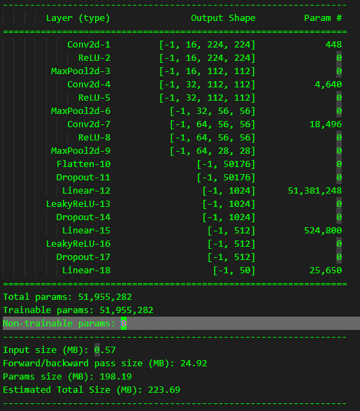
We can take a look at the model and each layer shapes plus number of parameters and some stats as below:
summary(cnn_model, (3, 224, 224))
Functions for train and test
In the train function we will pass the batches through the network and after each batch we will do a validation round. We will monitor both the training and validation loss. If the validation loss of the latest epoch is lower than the previous one, we will save the model. This will allow us to avoid saving a model that is overfitting. As mentioned earlier, if the validation loss does not change after 10 epochs, the learning rate will be decreased by the scheduler.
def train(n_epochs: int, loaders: dict, model: Any, optimizer: Any, scheduler: Any, loss_function: Any, use_cuda: bool, save_path: str) -> None:

    lowest_validation_loss = np.Inf

    print("Training on: ", device," -> ", torch.cuda.get_device_name(0))
    print('Memory Usage:')
    print('\tAllocated:', round(torch.cuda.memory_allocated(0)/1024**3,1), 'GB')
    print('\tCached:   ', round(torch.cuda.memory_reserved(0)/1024**3,1), 'GB')

    for epoch in range(1, n_epochs +1):
        train_loss, valid_loss = 0.0, 0.0

        ##Train model
        #Set model to train
        model.train()
        for batch_idx, (data, target) in enumerate(loaders['train']):
            #Move to GPU
            if use_cuda:
                data, target = data.cuda(), target.cuda()

                optimizer.zero_grad() #Clearing gradient
                output = model(data)
                loss = loss_function(output, target)
                loss.backward()
                optimizer.step()
                train_loss = train_loss + ((1 / (batch_idx + 1)) * (loss.data.item() - train_loss))
        print(f"Learning rate is now {optimizer.param_groups[0]['lr']}")

        #Evaluating model
        model.eval()
        for batch_idx, (data, target) in enumerate(loaders['validation']):
                #Move to GPU
                if use_cuda:
                    data, target = data.cuda(), target.cuda()
                output = model(data)
                loss = loss_function(output, target)
                valid_loss = valid_loss + ((1 / (batch_idx + 1)) * (loss.data.item() - valid_loss))

        train_loss = train_loss/len(train_loader)
        valid_loss = valid_loss/len(validation_loader)

        print(f'Epoch: {epoch} \tTraining Loss: {train_loss:.6f} \tValidation Loss: {valid_loss:.6f}')

        if (valid_loss <= lowest_validation_loss):
            print(f'Validation loss decreased ({lowest_validation_loss:.6f} --> {valid_loss:.6f}).  Saving model ...')
            torch.save(model.state_dict(), save_path)
            lowest_validation_loss = valid_loss

        scheduler.step(lowest_validation_loss)
    return model

def test(loaders: dict, model: Any, loss_function: Any) -> None:

    # monitor test loss and accuracy
    test_loss = 0.
    correct = 0.
    total = 0.

    # set the module to evaluation mode
    model.eval()

    for batch_idx, (data, target) in enumerate(loaders['test']):
        # move to GPU
        if device == "cuda":
            data, target = data.cuda(), target.cuda()
        # forward pass: compute predicted outputs by passing inputs to the model
        output = model(data)
        # calculate the loss
        loss = loss_function(output, target)
        # update average test loss
        test_loss = test_loss + ((1 / (batch_idx + 1)) * (loss.data.item() - test_loss))
        # convert output probabilities to predicted class
        pred = output.data.max(1, keepdim=True)[1]
        # compare predictions to true label
        correct += np.sum(np.squeeze(pred.eq(target.data.view_as(pred))).cpu().numpy())
        total += data.size(0)

    print('Test Loss: {:.6f}\n'.format(test_loss))

    print('\nTest Accuracy: %2d%% (%2d/%2d)' % (
        100. * correct / total, correct, total))
Time to train!
optimizer = get_optimizer(cnn_model, lr=0.01, momentum=0.9)

torch.cuda.empty_cache()

trained_model_scratch = train(60,
                        loaders_dict,
                        cnn_model,
                        optimizer,
                        get_scheduler(optimizer),
                        get_loss_function(),
                        True if device == "cuda" else False,
                        'cnn_scratch.pt')
The training will be for 60 epochs. Below the output while training is running:
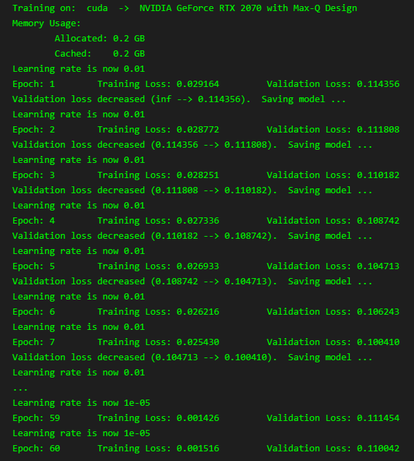
The model decreased the validation loss until epoch 20, after that it did not anymore.
Now that the model is trained and we have saved the best performant model, we can test it on the test dataset. These images the model has never seen before.
trained_model_scratch.load_state_dict(torch.load('cnn_scratch.pt'))
test(loaders_dict, trained_model_scratch, get_loss_function())
Output =>
Test Loss: 2.955963 Test Accuracy: 27% (345/1250)
The performance is not great as basically the model is recognizing only about a third of the test images. The model is very simple and sure, we could have done much better but what can we do to drastically improve the numbers almost immediately? Here is where transfer learning comes in handy.
Transfer Learning
Almost never you will want to train a whole CNN yourself. Modern CNN train on huge datasets like ImageNet taking weeks on multiple GPUs. With Transfer learning, we can use a pretrained network to fine tune it for our needs. For this implementation I selected ResNet50 which is a CNN that is 50 layers deep. This network was trained on ImageNet which has millions of images.
Load the model
from torchvision.models import resnet50, ResNet50_Weights
model_transfer = resnet50(weights=ResNet50_Weights.IMAGENET1K_V1)
The last layer of this network is called fc (Fully connected and has 1000 neurons). We will modify this layer to be outputting only 50 and we will freeze the weights.
for parameters in model_transfer.parameters():
    parameters.requires_grad = False

model_transfer.fc = nn.Sequential(nn.Linear(2048, 512),
                                    nn.ReLU(),
                                    nn.Dropout(0.15),
                                    nn.Linear(512, 50),
)

model_transfer.to(device)
Let’s train
optimizer = get_optimizer(model_transfer, lr=0.01, momentum=0.9)
trained_model_transfer_learning = train(50,
                        loaders_dict,
                        model_transfer,
                        optimizer,
                        get_scheduler(optimizer),
                        get_loss_function(),
                        True if device == "cuda" else False,
                        'cnn_transfer_learning.pt')
For this model we trained for 50 epochs. At epoch 48, which is the last time the model was saved, the validation loss was 0.030746
For the model from scratch, the best validation loss was 0.088764
Let’s test the model
model_transfer.load_state_dict(torch.load('cnn_transfer_learning.pt'))
test(loaders_dict, model_transfer, get_loss_function())
Output => Test Loss: 0.884768 Test Accuracy: 77% (970/1250)
Wow, the improvement is noticeable and we did not really do much to get these numbers. The model is ~3 times more accurate.
Inference time
Let’s do some inference and see what are the results on some random image. We will take the top 5 predictions of an image and see which are the corresponding labels.
def predict_landmarks(img_path, k):
    top_k_classes = []
    img = Image.open(img_path)
    convert_to_tensor = transforms.Compose([transforms.Resize([224,224]),
                                     transforms.ToTensor()])
    img = convert_to_tensor(img)
    img.unsqueeze_(0)

    img = img.to(device)

    model_transfer.eval()
    output = model_transfer(img)
    value, index_class = output.topk(k)

    for index in index_class[0].tolist():
        top_k_classes.append(classes[index])

    model_transfer.train()

    return value[0].tolist(), top_k_classes


predict_landmarks('data/landmark_images/test/09.Golden_Gate_Bridge/1bc7a7f05288153b.jpg', 5)
Output => ([16.725576400756836, 10.52921199798584, 10.092767715454102, 8.731866836547852, 7.1621599197387695], [‘Golden Gate Bridge’, ‘Forth Bridge’, ‘Brooklyn Bridge’, ‘Dead Sea’, ‘Niagara Falls’])
Well done, the image in input was from the Golden Gate Bridge and the prediction with highest % is indeed the Golden Gate Bridge.
The full notebook with code can be found here