Convolutional Neural Networks for Audio Signal Analysis

This post is an implementation for the Z by HP Unlocked Challenge 3 - Signal Processing on Kaggle.

Scope

The scope of this challenge is to be able to identify Capuchin Bird calls within a given forest audio.

Here is our guy:

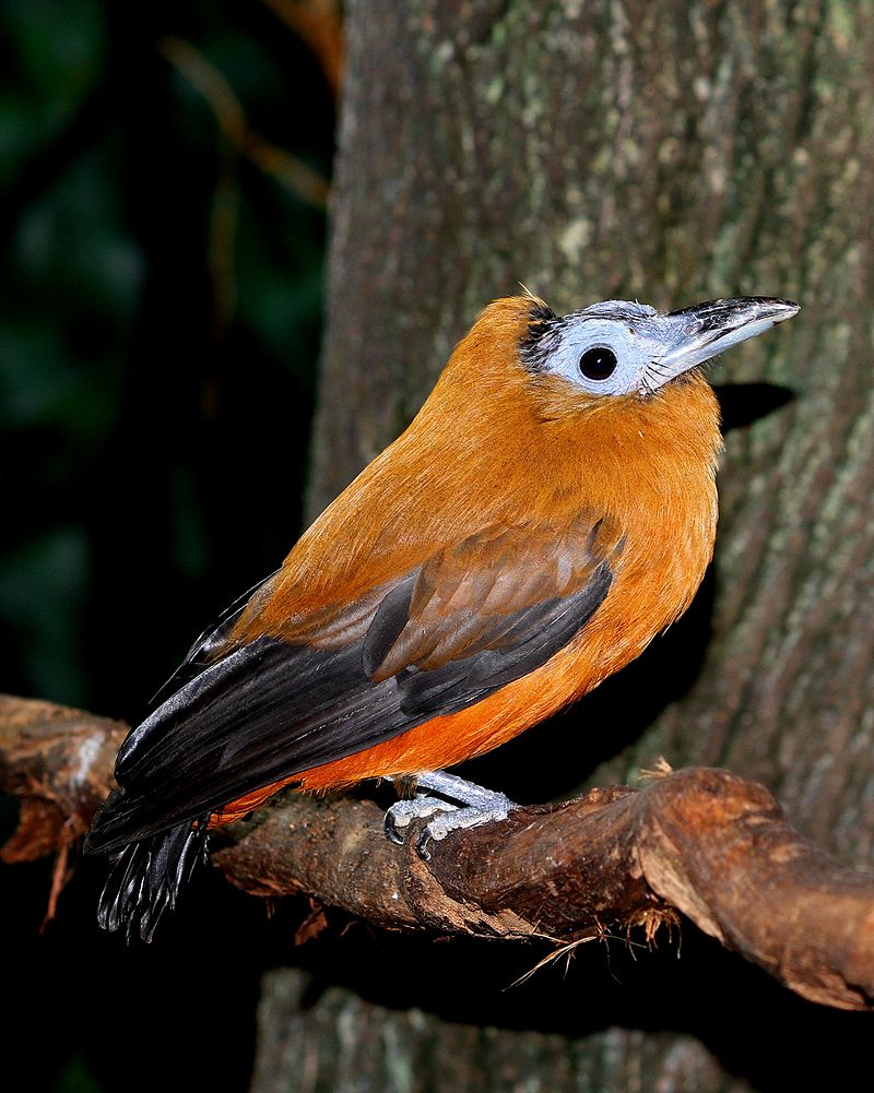
Picture from Wikipedia

Plan of attack

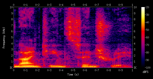
The main idea is to obtain a visual representation of the audio into a spectrogram which will then be fed to a CNN that will be able to distinguish whether the image fed in input is a capuchin bird call or something else.

Example of a Spectrogram (Wikipedia)

The challenge is divided into two parts. First we will need to be able to build a model that can identify the calls correctly, then we will need to use the model to count the calls within a long forest audio. The dataset is divided into three splits:

• Parsed Capuchin bird => A collection of capuchin bird calls only. Short clips.
• Parse Non Capuchin bird => A collection of other sounds from the forest/animals. Short clips.
• Forest Recording => A collection of long audios. In these audios there may or may not be capuchin birds calls. Long clips.

Code Implementation

#Imports

import tensorflow as tf
import tensorflow_io as tfio
from matplotlib import pyplot as plt
import os, csv
import IPython as IPD
from IPython.display import YouTubeVideo
from tensorflow.keras.models import Sequential
from tensorflow.keras.layers import Conv2D, Dense, Flatten, MaxPool2D, Dropout
from itertools import groupby

#Let's check how our guy sounds like

YouTubeVideo("cwHWpq79MCM")

![Watch the video]

Data location and variables

#Data Folder. The original dataset is taken from Kaggle: https://www.kaggle.com/datasets/kenjee/z-by-hp-unlocked-challenge-3-signal-processing?resource=download
ROOT = "data"
capuchin_data = os.path.join(ROOT, "Parsed_Capuchinbird_Clips")
other_data = os.path.join(ROOT, "Parsed_Not_Capuchinbird_Clips")
forest_data = os.path.join(ROOT, "Forest_Recordings")

DOWNSAMPLE_RATE = 16000
EPOCHS = 10
EXAMPLE_FILE_CAPUCHIN = os.path.join(capuchin_data, "XC16803-1.wav")
EXAMPLE_FILE_NOT_CAPUCHIN = os.path.join(other_data, "afternoon-birds-song-in-forest-2.wav")

Functions and Exploration

#Downsampling data from 44.1khz to xxx khz. It will be lighter for processing
def downsample_audio(filename, downsampling_rate, is_forest=False):
  file, to_tensor, sample_rate, wav = "","", "",""
  if is_forest:
    file = tfio.audio.AudioIOTensor(filename)
    to_tensor = file.to_tensor()
    to_tensor = tf.math.reduce_sum(to_tensor, axis=1) /2
    sample_rate = tf.cast(file.rate, dtype=tf.int64)
    wav = tfio.audio.resample(to_tensor, rate_in=sample_rate, rate_out=downsampling_rate)
  else:
    file = tf.io.read_file(filename)
    wav, sample_rate = tf.audio.decode_wav(file, desired_channels=1)
    wav = tf.squeeze(wav, axis=-1)
    sample_rate = tf.cast(sample_rate, dtype=tf.int64)
    wav = tfio.audio.resample(wav, rate_in=sample_rate, rate_out=downsampling_rate)
  
  return wav

#Function to return spectrogram to be fed to model. Audio will be padded if shorter than selected length
def preprocess_data(file_path, label):
  file_audio = downsample_audio(file_path, DOWNSAMPLE_RATE)
  file_audio = file_audio[:selected_length]
  zero_padding = tf.zeros([selected_length] - tf.shape(file_audio), dtype=tf.float32)
  file_audio = tf.concat([zero_padding, file_audio], 0)
  spectrogram = tf.abs(tf.signal.stft(file_audio, frame_length=320, frame_step=32))
  spectrogram = tf.expand_dims(spectrogram, axis=2)
  return spectrogram, label

#Function to return spectrogram for forest data (mp3)
def preprocess_data_full_audio(sample, label):
  file_audio = sample[0]
  zero_padding = tf.zeros([selected_length] - tf.shape(file_audio), dtype=tf.float32)
  file_audio = tf.concat([zero_padding, file_audio], 0)
  spectrogram = tf.abs(tf.signal.stft(file_audio, frame_length=320, frame_step=32))
  spectrogram = tf.expand_dims(spectrogram, axis=2)
  return spectrogram, label

#Playing some audio examples
  
IPD.display.Audio(EXAMPLE_FILE_CAPUCHIN)
  
IPD.display.Audio(EXAMPLE_FILE_NOT_CAPUCHIN)
  
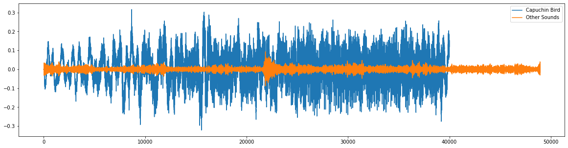
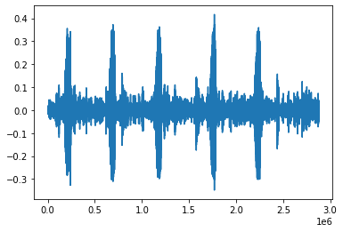
#Downsample and plot
plt.figure(figsize=(20,5))
plt.plot(downsample_audio(EXAMPLE_FILE_CAPUCHIN, DOWNSAMPLE_RATE))
plt.plot(downsample_audio(EXAMPLE_FILE_NOT_CAPUCHIN, DOWNSAMPLE_RATE))
plt.legend(['Capuchin Bird', 'Other Sounds'])
plt.show()

Stats on the capuchin bird data

lengths = []

for file in os.listdir(capuchin_data):
  downsampled_audio = downsample_audio(os.path.join(capuchin_data, file), DOWNSAMPLE_RATE)
  lengths.append(len(downsampled_audio))

print(f"Longest call of the capuchin bird is {max(lengths)/DOWNSAMPLE_RATE} seconds")
print(f"Shortest call of the capuchin bird is {min(lengths)/DOWNSAMPLE_RATE} seconds")
print(f"Average call of the capuchin bird is {round(sum(lengths)/len(lengths))/DOWNSAMPLE_RATE} seconds")

Longest call of the capuchin bird is 5.0 seconds Shortest call of the capuchin bird is 2.0 seconds Average call of the capuchin bird is 3.3848125 seconds We can take the average as ballpark which is ~54000

selected_length = int(round(sum(lengths)/len(lengths),-3))

#Loading all data
pos = tf.data.Dataset.list_files(capuchin_data+'/*.wav')
neg = tf.data.Dataset.list_files(other_data+'/*.wav')

#Creating Labels 1 for POS and 0 for NEG of the same lenghts of the datasets
pos_dataset = tf.data.Dataset.zip((pos, tf.data.Dataset.from_tensor_slices(tf.ones(len(pos)))))
neg_dataset = tf.data.Dataset.zip((neg, tf.data.Dataset.from_tensor_slices(tf.zeros(len(neg)))))
full_data = pos_dataset.concatenate(neg_dataset)

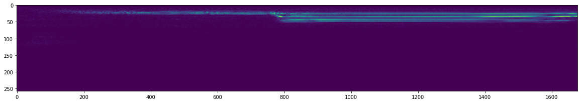
Plotting Spectrogram Examples Audios (Capuchin and then Other Sounds)

filepath, label = pos_dataset.shuffle(buffer_size=1000).as_numpy_iterator().next()
spectrogram , label = preprocess_data(filepath, label)
plt.figure(figsize=(20,5))
plt.imshow(tf.transpose(spectrogram)[0])
plt.show()

filepath, label = neg_dataset.shuffle(buffer_size=10000).as_numpy_iterator().next()
spectrogram , label = preprocess_data(filepath, label)
plt.figure(figsize=(20,5))
plt.imshow(tf.transpose(spectrogram)[0])
plt.show()

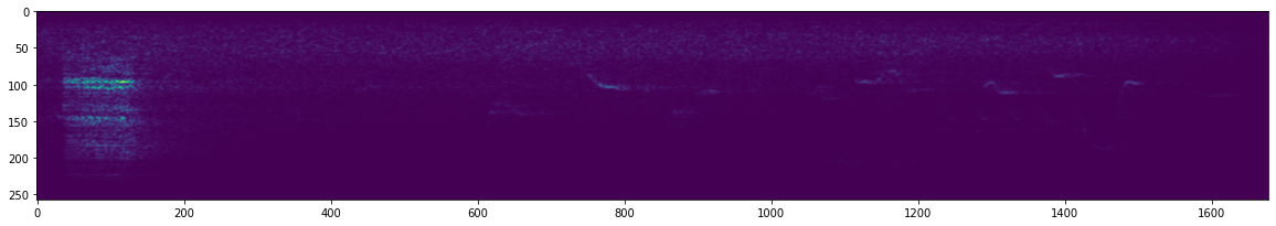
Spectrograms will be fed to the CNN and will try to identify the Capuchin bird from the image representation of the sound.

Preparing Data Pipeline and Data Splits

#Data Pipeline
full_data_pipeline = full_data.map(preprocess_data).cache().shuffle(buffer_size=1000).batch(16).prefetch(8)
total = int(len(full_data_pipeline))
train_data = full_data_pipeline.take(int(total*0.7))
val_data = full_data_pipeline.skip(int(total*0.7)).take(int(total*0.1))
test_data = full_data_pipeline.skip(int(total*0.7)).skip(int(total*0.1)).take(int(total*0.2))

print('Training batch size', len(train_data))
print('Validation batch size', len(val_data))
print('Test batch size', len(test_data))

Training batch size 35

Validation batch size 5

Test batch size 10

Each batch will have 16 samples.

Let’s take a look at the shape of the samples.

samples, labels = train_data.as_numpy_iterator().next()
samples.shape

(16, 1678, 257, 1)

Model

model = Sequential()
model.add(Conv2D(16, (3, 3), activation='relu', input_shape=(1678, 257, 1)))
model.add(MaxPool2D(pool_size=3, strides=2, padding='same'))
model.add(Conv2D(16, (3, 3), activation='relu'))
model.add(MaxPool2D(pool_size=3, strides=2, padding='same'))
model.add(Flatten())
model.add(Dense(128, activation='relu'))
model.add(Dropout(0.3))
model.add(Dense(1, activation='sigmoid'))
model.compile('Adam', loss='BinaryCrossentropy', metrics=[tf.keras.metrics.Recall(),tf.keras.metrics.Precision()])

model.summary()

Model: “sequential_1” _________________________ Layer (type) Output Shape Param #
================================================================= conv2d_2 (Conv2D) (None, 1676, 255, 16) 160

max_pooling2d_2 (MaxPooling (None, 838, 128, 16) 0
2D)

conv2d_3 (Conv2D) (None, 836, 126, 16) 2320

max_pooling2d_3 (MaxPooling (None, 418, 63, 16) 0
2D)

flatten_1 (Flatten) (None, 421344) 0

dense_2 (Dense) (None, 128) 53932160

dropout (Dropout) (None, 128) 0

dense_3 (Dense) (None, 1) 129

================================================================= Total params: 53,934,769 Trainable params: 53,934,769 Non-trainable params: 0

Time to train

hist = model.fit(train_data, epochs=10, validation_data=test_data, callbacks=tf.keras.callbacks.EarlyStopping(verbose=1, 
                                               patience=5,
                                               restore_best_weights=True
                                              ),)

Epoch 1/10 35/35 [==============================] - 58s 2s/step - loss: 2.5330 - recall_1: 0.8714 - precision_1: 0.7871 - val_loss: 0.2347 - val_recall_1: 0.8980 - val_precision_1: 0.9362 Epoch 2/10 35/35 [==============================] - 59s 2s/step - loss: 0.2148 - recall_1: 0.9128 - precision_1: 0.9444 - val_loss: 0.0367 - val_recall_1: 0.9545 - val_precision_1: 1.0000 Epoch 3/10 35/35 [==============================] - 58s 2s/step - loss: 0.0384 - recall_1: 0.9799 - precision_1: 0.9865 - val_loss: 0.0104 - val_recall_1: 1.0000 - val_precision_1: 1.0000 Epoch 4/10 35/35 [==============================] - 58s 2s/step - loss: 0.0114 - recall_1: 1.0000 - precision_1: 1.0000 - val_loss: 0.0075 - val_recall_1: 0.9756 - val_precision_1: 1.0000 Epoch 5/10 35/35 [==============================] - 61s 2s/step - loss: 0.0034 - recall_1: 1.0000 - precision_1: 1.0000 - val_loss: 0.0018 - val_recall_1: 1.0000 - val_precision_1: 1.0000 Epoch 6/10 35/35 [==============================] - 58s 2s/step - loss: 0.0094 - recall_1: 0.9935 - precision_1: 1.0000 - val_loss: 0.0041 - val_recall_1: 1.0000 - val_precision_1: 1.0000 Epoch 7/10 35/35 [==============================] - 58s 2s/step - loss: 0.0037 - recall_1: 0.9935 - precision_1: 1.0000 - val_loss: 6.3050e-04 - val_recall_1: 1.0000 - val_precision_1: 1.0000 Epoch 8/10 35/35 [==============================] - 58s 2s/step - loss: 0.0013 - recall_1: 1.0000 - precision_1: 1.0000 - val_loss: 2.9292e-04 - val_recall_1: 1.0000 - val_precision_1: 1.0000 Epoch 9/10 35/35 [==============================] - 59s 2s/step - loss: 7.6782e-04 - recall_1: 1.0000 - precision_1: 1.0000 - val_loss: 1.4974e-04 - val_recall_1: 1.0000 - val_precision_1: 1.0000 Epoch 10/10 35/35 [==============================] - 58s 2s/step - loss: 4.6571e-04 - recall_1: 1.0000 - precision_1: 1.0000 - val_loss: 1.3740e-04 - val_recall_1: 1.0000 - val_precision_1: 1.0000

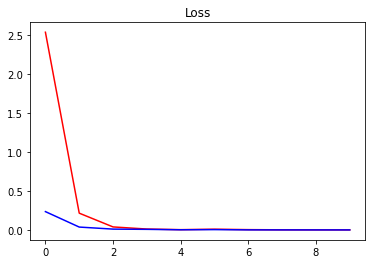
Plotting some stats from the training

plt.title("Loss")
plt.plot(hist.history["loss"], "r")
plt.plot(hist.history["val_loss"], "b")
plt.show()

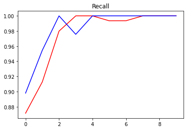
plt.title("Recall")
plt.plot(hist.history["recall_1"], "r")
plt.plot(hist.history["val_recall_1"], "b")
plt.show()

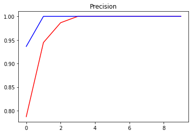
plt.title("Precision")
plt.plot(hist.history["precision_1"], "r")
plt.plot(hist.history["val_precision_1"], "b")
plt.show()

Testing against Test Dataset

test_audio = []
test_labels = []
cnt = 0

for X_test, y_test in test_data.as_numpy_iterator():

    y_hat = model.predict(X_test)
    y_hat = [1 if prediction > 0.5 else 0 for prediction in y_hat]
    print(f'Predicted labels: {y_hat}')
    print(f'True labels: {y_test}')
    for idx, item in enumerate(y_hat):
        if item == y_test[idx]:
            cnt+=1
    print(f'Accuracy is {(cnt/16)*100} %')
    cnt = 0

Output exceeds the size limit. Open the full output data in a text editor 1/1 [==============================] - 23s 23s/step Predicted labels: [0, 1, 0, 1, 0, 0, 0, 0, 0, 1, 0, 0, 0, 0, 0, 0] True labels: [0. 1. 0. 1. 0. 0. 0. 0. 0. 1. 0. 0. 0. 0. 0. 0.] Accuracy is 100.0 1/1 [==============================] - 23s 23s/step Predicted labels: [1, 0, 0, 0, 0, 0, 0, 1, 1, 0, 0, 0, 0, 0, 0, 0] True labels: [1. 0. 0. 0. 0. 0. 0. 1. 1. 0. 0. 0. 0. 0. 0. 0.] Accuracy is 100.0 1/1 [==============================] - 21s 21s/step Predicted labels: [0, 0, 0, 1, 0, 0, 0, 0, 0, 0, 0, 1, 0, 0, 0, 1] True labels: [0. 0. 0. 1. 0. 0. 0. 0. 0. 0. 0. 1. 0. 0. 0. 1.] Accuracy is 100.0 1/1 [==============================] - 22s 22s/step Predicted labels: [0, 0, 0, 1, 0, 0, 0, 0, 1, 1, 0, 0, 0, 0, 0, 1] True labels: [0. 0. 0. 1. 0. 0. 0. 0. 1. 1. 0. 0. 0. 0. 0. 1.] Accuracy is 100.0 1/1 [==============================] - 21s 21s/step Predicted labels: [0, 0, 0, 1, 0, 0, 1, 0, 0, 0, 0, 0, 0, 1, 1, 0] True labels: [0. 0. 0. 1. 0. 0. 1. 0. 0. 0. 0. 0. 0. 1. 1. 0.] Accuracy is 100.0 1/1 [==============================] - 23s 23s/step Predicted labels: [0, 1, 0, 0, 0, 0, 1, 0, 1, 0, 1, 0, 1, 0, 0, 0] True labels: [0. 1. 0. 0. 0. 0. 1. 0. 1. 0. 1. 0. 1. 0. 0. 0.] Accuracy is 100.0 1/1 [==============================] - 22s 22s/step … 1/1 [==============================] - 21s 21s/step Predicted labels: [0, 0, 0, 0, 0, 0, 1, 0, 0, 0, 1, 0, 1, 1, 1, 0] True labels: [0. 0. 0. 0. 0. 0. 1. 0. 0. 0. 1. 0. 1. 1. 1. 0.] Accuracy is 100.0

It seems that the model is identifying quite well the capuchin bird calls. Let’s dive more into the data.

Working with full audio (Forest recording)

The idea here is that from a full audio of 3 min, we will need to count how many times the capuchin bird is heard. To do this we will need to split the full audio into chunks and analyze each chunk and tell whether the capuchin bird is heard or not. Once predictions are done on 1 file. We will need to check if 1s (predicted True) are consecutive. If there are consecutives ones, then it means that is just 1 call. E.g. 1, 0, 1, 1, 1, 0, 0, 1 => Total is 3 and not 5. This is because we are splitting the audio into slides, windows.

detections = {}

#Iterating through the folder of forest data. Splitting into windows and feeding to the model
for file in os.listdir(forest_data):
  file_path = os.path.join(forest_data, file)

  wav = downsample_audio(file_path, DOWNSAMPLE_RATE, is_forest=True)
  #Splitting into subsequences
  wav_slices = tf.keras.utils.timeseries_dataset_from_array(wav, wav, sequence_length=selected_length, sequence_stride=selected_length, batch_size=1)
  wav_slices = wav_slices.map(preprocess_data_full_audio)
  wav_slices = wav_slices.batch(32)

  yhat = model.predict(wav_slices)
  detections[file] = yhat

#Converting logits to 1s and 0s
final_preds= {}
for file, logits in detections.items():
  final_preds[file] = [1 if prediction > 0.99 else 0 for prediction in logits]

combined_preds = {}
for file, converted_logits in final_preds.items():
  combined_preds[file] = tf.math.reduce_sum([key for key, group in groupby(converted_logits)]).numpy()

combined_preds

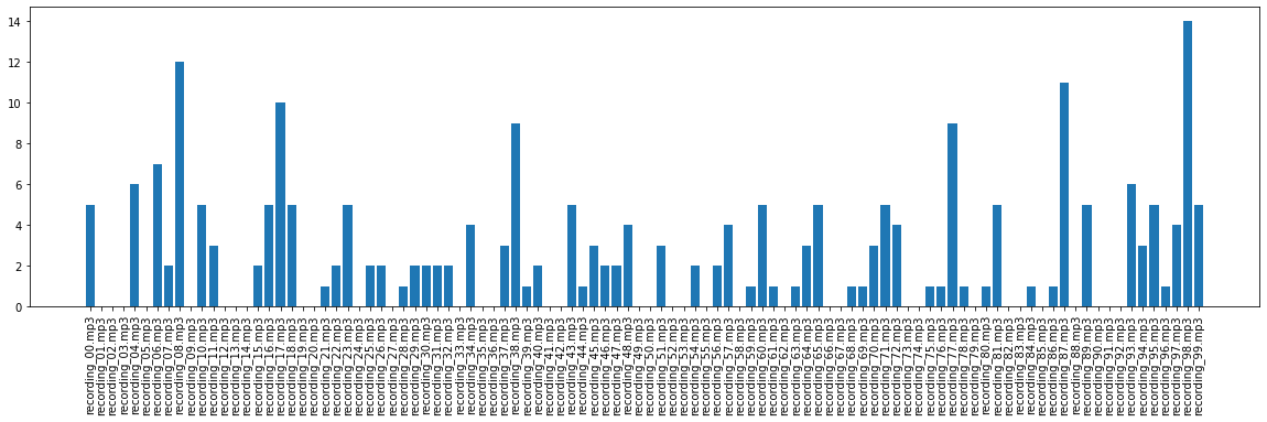
List of counts per file:

‘recording_00.mp3’: 5, ‘recording_01.mp3’: 0, ‘recording_02.mp3’: 0, ‘recording_03.mp3’: 0, ‘recording_04.mp3’: 6, ‘recording_05.mp3’: 0, ‘recording_06.mp3’: 7, ‘recording_07.mp3’: 2, ‘recording_08.mp3’: 12, ‘recording_09.mp3’: 0, ‘recording_10.mp3’: 5, ‘recording_11.mp3’: 3, ‘recording_12.mp3’: 0, ‘recording_13.mp3’: 0, ‘recording_14.mp3’: 0, ‘recording_15.mp3’: 2, ‘recording_16.mp3’: 5, ‘recording_17.mp3’: 10, ‘recording_18.mp3’: 5, ‘recording_19.mp3’: 0, ‘recording_20.mp3’: 0, ‘recording_21.mp3’: 1, ‘recording_22.mp3’: 2, ‘recording_23.mp3’: 5, ‘recording_24.mp3’: 0, … ‘recording_95.mp3’: 5, ‘recording_96.mp3’: 1, ‘recording_97.mp3’: 4, ‘recording_98.mp3’: 14, ‘recording_99.mp3’: 5

max_count = max([value for value in combined_preds.values()])
print(f'Max count in a single forest file is {max_count}')

Max count in a single forest file is 14 Which files?

file_names = []
sep = ','
for k, v in combined_preds.items():
    if v == max_count:
        file_names.append(k)
print(f'Files with max count are {sep.join(file_names)}')

Files with max count are recording_98.mp3

Visualize Predictions

names = list(combined_preds.keys())
values = list(combined_preds.values())
plt.figure(figsize=(20,5))
plt.xticks(rotation='vertical')
plt.bar(range(len(combined_preds)), values, tick_label=names)
plt.show()

plt.plot(downsample_audio(os.path.join(forest_data, "recording_98.mp3"), DOWNSAMPLE_RATE, is_forest=True))
plt.figure(figsize=(30,10))
plt.show()

IPD.display.Audio(os.path.join(forest_data, "recording_98.mp3"))

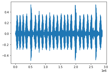
It seems that there more than just 14 calls in file recording_98. Let’s check some random audio where no detection was observed.

plt.plot(downsample_audio(os.path.join(forest_data, "recording_01.mp3"), DOWNSAMPLE_RATE, is_forest=True))
plt.figure(figsize=(30,10))
plt.show()

This was one was correct.

Let’s check if a random file has the right detected # of calls

import random
n = str(random.randint(1,len(detections))).zfill(2)
plt.plot(downsample_audio(os.path.join(forest_data, "recording_"+n+".mp3"), DOWNSAMPLE_RATE, is_forest=True))
plt.title("recording_"+n+".mp3")
plt.figure(figsize=(30,10))
plt.show()

calls = combined_preds["recording_"+n+".mp3"]
print(f"Number of calls identified {calls}")

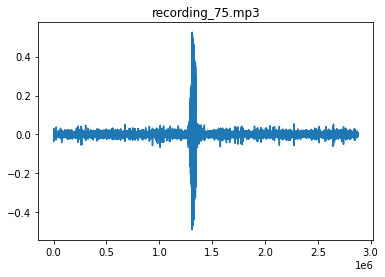
Number of calls identified 1

The above is correct too.

Another file.

calls = combined_preds["recording_00.mp3"]
print(f"Number of calls identified {calls}")

Number of calls identified 5

plt.plot(downsample_audio(os.path.join(forest_data, "recording_00.mp3"), DOWNSAMPLE_RATE, is_forest=True))
plt.figure(figsize=(30,10))
plt.show()

This one is correct as well.

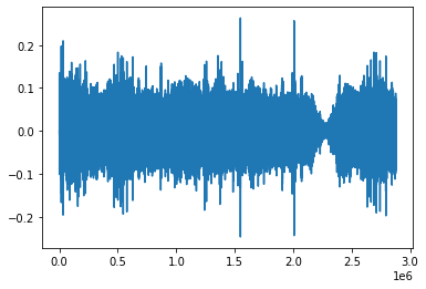
One interesting audio was #89.

plt.plot(downsample_audio(os.path.join(forest_data, "recording_89.mp3"), DOWNSAMPLE_RATE, is_forest=True))
plt.figure(figsize=(30,10))
plt.show()

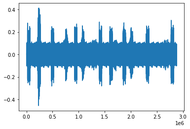
File 89 was identified correctly although based on the waveform looks like there would be more calls than just 5. Some calls are very low but still identified by the model. For audios with high density calls the model does not perform perfectly. Probably having more balanced data and/or changing a bit the model architecture could help identify better. Maybe even having a different window would be beneficial, above was used 54000.

POSSIBLE IMPROVEMENTS

• Add data augmentation
• Different Model Architecture
• Transfer Learning with YAMNET as suggested by ![Watch the video] by Ken Jee

---

<

Previous Post

DCGAN - GENERATE FACES

>

Next Post

Accelerate Pandas for quicker data manipulation