Quantization: A Crucial Technique in Today’s AI Landscape
In this blog post, we will discuss about a topic of significant importance in the current AI scene. When discussing model size, we are referring to the number of parameters a given model possesses. For instance, the current largest Llama 3 model boasts 70 billion parameters, and an even larger one, still in the training phase at the time of this post, is expected to have around 400 billion parameters.
Such immense models pose a challenge when it comes to deployment on consumer-grade hardware, as the entirety of the parameters must be loaded into memory during the inference process. This is where the technique of Quantization proves to be indispensable.
What is Quantization?
Quantization is a technique used to reduce the size of a model, making it more feasible to deploy on resource-constrained hardware. In essence, quantization involves reducing the number of bits required to represent each parameter within the model.
The most common approach to quantization is to convert floating-point numbers to integers. This process not only results in a smaller model size but also has the added benefit of increased speed. For instance, multiplying integer values is computationally faster than multiplying floating-point numbers.
However, it is important to note that quantization is not without its drawbacks. One of the primary concerns is the potential loss of precision, which may negatively impact the model’s performance. Therefore, striking the right balance between model size, speed, and precision is crucial when employing quantization techniques.
Data Types
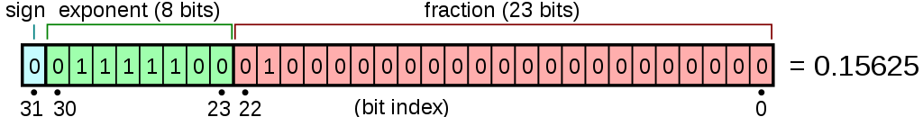
Let’s begin by understanding what floating-point numbers are and how they are represented. A commonly used floating-point format is FP32, also known as single-precision floating-point. FP32 is represented using 32 bits, which are further divided into three parts:
- First bit is the sign (0 being positive)
- Next 8 bit is the exponent, the range of the number
- Last 23 bit is the fraction, precision of the number
Example from Wikipedia
There are other floating-point formats besides FP32, such as FP16 (16-bit half-precision), FP64 (64-bit double-precision), and BF16 (Brain Floating Point), which is a 16-bit format designed for deep learning applications. Each of these formats has its own trade-offs between precision, range, and memory usage.
In contrast to floating-point numbers, integers can be either signed or unsigned and are available in different bit-widths. The common bit-widths for integers are:
8-bit: This can represent signed values in the range of -128 to 127 or unsigned values from 0 to 255. 16-bit, 32-bit and 64-bit are also available.
In PyTorch, the following integer tensor types are available:
torch.int8 (8-bit signed integers) torch.int16 (16-bit signed integers) torch.int32 (32-bit signed integers) torch.int64 (64-bit signed integers) torch.uint8 (8-bit unsigned integers)
You can look at the ranges by using torch.iinfo(torch.int8) for example => iinfo(min=0, max=255, dtype=uint8)
So why bringing up this distinction? Simply put the main purpose of bringing up the distinction between floating-point numbers and integers is to highlight the core concept of quantization. Quantization aims to reduce the number of bits required to represent the values in a model, and so to a smaller range of integer values. The end-result is a reduced memory footprint and potentially accelerating computations. By converting floating-point numbers to integers, quantization takes advantage of the more compact and computationally efficient nature of integers.
Where Quantization is applied
In a simple neural network composed of stacked linear layers, each layer consists of matrices, namely weight and bias matrices. These matrices typically store their values in floating-point format to maintain high precision. This is where quantization comes into play, aiming to convert the floating-point values to integers.
The quantization process in a neural network involves the following steps for each layer:
-
Quantize the input: Convert the floating-point input values to integer values.
-
Quantize the weights and biases: Convert the floating-point weight and bias values to integer values.
-
Perform the calculation: Execute the matrix multiplications and other operations using the quantized integer values.
-
Dequantize the output: Convert the integer output values back to floating-point values, which can then be fed to the next layer.
Here’s a visual example:
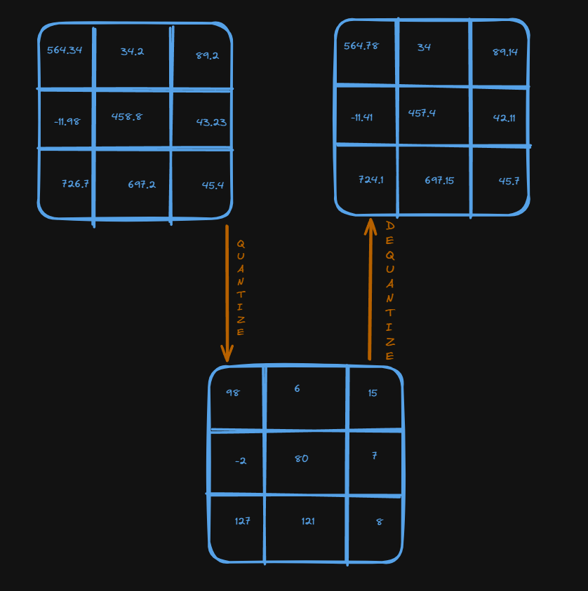
The above is just an example of how a matrix that has floating point values is quantized to a range between -128 to 127. The same is the dequantized. In the original matrix, each value takes up 4 bytes, so 32 bit. In the quantized matrix each value takes up 8 bit. You can see that some values have slightly changed, meaning we lost some precision. so the model will not be as accurate as the not quantized one.
In terms of value ranges, there are two types of quantization: asymmetric and symmetric.
Asymmetric quantization maps floating-point values to unsigned integer values, typically in the range of 0 to 255 (for 8-bit quantization). This type of quantization is well-suited for data with a non-zero minimum value or where the zero value has a special meaning.
Symmetric quantization maps floating-point values to signed integer values, typically in the range of -127 to 127 (for 8-bit quantization). In this case, the zero value in the original matrix or tensor remains zero after quantization
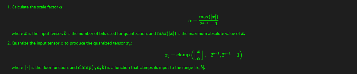
Symmetric Quantization
The symmetric quantization process can be expressed as follows:
Now, let’s see in code how this works.
import torch

original_tensor = torch.randn(10) * 200 + 50
print(f"Max value: {original_tensor.max()}")
print(f"Min value: {original_tensor.min()}")

#Set 0 as first element
original_tensor[0] = 0
Output:
Max value: 376.07928466796875
Min value: -194.05178833007812
Let’s look at the tensor:
tensor([   0.0000,   -7.2955, -174.8314, -194.0518,  174.6870,  376.0793,
         -29.7248, -143.4094,  260.2398,  -57.8868])
Based on the formula for the Symmetric Quantization, we need a clamp function:
def clamp(params_q: torch.Tensor, lower_bound: float, upper_bound: float) -> torch.Tensor:
    """
    Clamp all elements in the tensor to a minimum and maximum value.

    Args:
        params_q (torch.Tensor): The input tensor.
        lower_bound (float): The minimum value.
        upper_bound (float): The maximum value.

    Returns:
        torch.Tensor: A tensor with the same shape as `params_q` where all elements are in the range [`lower_bound`, `upper_bound`].
    """
    return torch.clamp(params_q, lower_bound, upper_bound)
And let’s write the symetric quantization which will return the quantized tensor and the scale
def symmetric_quantization(params: torch.Tensor, bits: int) -> tuple[torch.Tensor, float]:
    """
    Quantize the input tensor using symmetric quantization.

    Args:
        params (torch.Tensor): The input tensor.
        bits (int): The number of bits to use for quantization.

    Returns:
        tuple[torch.Tensor, float]: A tuple containing the quantized tensor and the scale factor.
    """
    alpha = torch.max(torch.abs(params))
    scale = alpha / (2**(bits-1)-1)
    lower_bound = -2**(bits-1)
    upper_bound = 2**(bits-1)-1
    quantized = clamp(torch.round(params / scale), lower_bound, upper_bound).long()
    return quantized, scale
Now let’s call the symmetric_quantization function and pass the tensor and the bits as 8:
symmetric_q_tensor, symmetric_scale = symmetric_quantization(original_tensor, 8)
This results into:
Symmetric scale: 2.961254119873047
tensor([  0,  -2, -59, -66,  59, 127, -10, -48,  88, -20])
Here the 0 remains the same as in the original tensor.
How about going back, dequantize the tensor? Let’s write a small function for it:
def symmetric_dequantize(params_q: torch.Tensor, scale: float) -> torch.Tensor:
    """
    Dequantize the input tensor using symmetric dequantization.

    Args:
        params_q (torch.Tensor): The input tensor.
        scale (float): The scale factor.

    Returns:
        torch.Tensor: The dequantized tensor.
    """
    return params_q.float() * scale
When calling this function with the symmetric_q tensor, we get back this:
deq_tensor = symmetric_dequantize(symmetric_q_tensor, symmetric_scale)
 tensor([   0.0000,   -5.9225, -174.7140, -195.4428,  174.7140,  376.0793,
         -29.6125, -142.1402,  260.5904,  -59.2251])
Let’s put this dequantized and original tensors close to each other:
Original: tensor([   0.0000,   -7.2955, -174.8314, -194.0518,  174.6870,  376.0793,
         -29.7248, -143.4094,  260.2398,  -57.8868])

Dequantized_symmetric:  tensor([   0.0000,   -5.9225, -174.7140, -195.4428,  174.7140,  376.0793,
         -29.6125, -142.1402,  260.5904,  -59.2251])
Here you can see some numbers match, some are different. Let’s calculate the quantization error:
def quantization_error(original_tensor: torch.Tensor, deq_tensor: torch.Tensor) -> float:
    """
    Calculate the mean squared error between the original and the dequantized values.

    Args:
        original_tensor (torch.Tensor): The original tensor.
        deq_tensor (torch.Tensor): The dequantized tensor.

    Returns:
        float: The mean squared error.
    """
    return torch.mean((original_tensor - deq_tensor)**2)
And let’s call it
q_error = quantization_error(original_tensor, deq_tensor)


0.7371761798858643
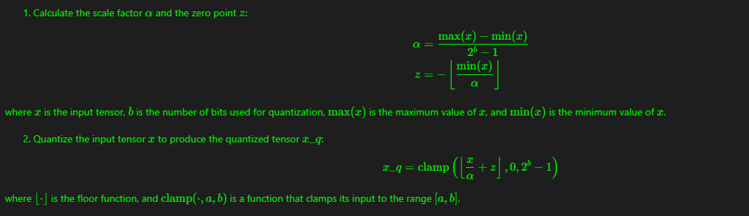
Asymmetric Quantization
The asymmetric quantization process can be expressed as follows:
As for the symmetric quantization, let’s see how to implement it in code
def asymmetric_quantization(params: torch.Tensor, bits: int) -> tuple[torch.Tensor, float, int]:
    """
    Quantize the input tensor using asymmetric quantization.

    Args:
        params (torch.Tensor): The input tensor.
        bits (int): The number of bits to use for quantization.

    Returns:
        tuple[torch.Tensor, float, int]: A tuple containing the quantized tensor, the scale factor, and the zero point.
    """
    alpha = params.max()
    beta = params.min()
    scale = (alpha - beta) / (2**bits-1)
    zero = -1*torch.round(beta / scale)
    lower_bound, upper_bound = 0, 2**bits-1
    quantized = clamp(torch.round(params / scale + zero), lower_bound, upper_bound).long()
    return quantized, scale, zero
This function will return the quantized tensor, the scale and the zero. For the clamp we use the same function as before.
Let’s run the function with the same original tensor:
asymmetric_q_tensor, asymmetric_scale, asymmetric_zero = asymmetric_quantization(original_tensor, 8)
Which results into the below:
Asymmetric scale: 2.2358081340789795,
Zero: 87
tensor([ 87,  84,   9,   0, 165, 255,  74,  23, 203,  61])
Here you can see that the 0 is not anymore 0 but 87. The max value is 255.
As for the symmetric quantization, let’s dequantized the asymmetric quantized tensor:
def asymmetric_dequantize(asym_q_tensor: torch.Tensor, scale: float, zero: int) -> torch.Tensor:
    """
    Dequantize the input tensor using asymmetric dequantization.

    Args:
        asym_q_tensor (torch.Tensor): The input tensor.
        scale (float): The scale factor.
        zero (int): The zero point.

    Returns:
        torch.Tensor: The dequantized tensor.
    """
    return (asym_q_tensor.float() - zero) * scale
And call it on the asymmetric quantized tensor and put it next to the original tensor:
deq_tensor = asymmetric_dequantize(asymmetric_q_tensor, asymmetric_scale, asymmetric_zero)
Original: tensor([   0.0000,   -7.2955, -174.8314, -194.0518,  174.6870,  376.0793,
         -29.7248, -143.4094,  260.2398,  -57.8868])

Dequantized_Asymmetric: tensor([   0.0000,   -6.7074, -174.3930, -194.5153,  174.3930,  375.6158,
         -29.0655, -143.0917,  259.3537,  -58.1310])
Also in this case some values match and some are a bit different. Let’s calculate the error:
q_error = quantization_error(original_tensor, deq_tensor)

0.24344968795776367
Common Quantization Techniques
Below are listed common quantization techniques briefly explained.
QAT (Quantization Aware Training)
QAT involves simulating quantization during the training process, allowing the model to learn to be robust to the quantization noise. This method typically provides better performance compared to PTQ, especially in terms of maintaining model accuracy after quantization. Both symmetric and asymmetric quantization can be utilized in QAT.
PTQ (Post Training Quantization)
PTQ involves quantizing a pre-trained model without further training. This method is typically used for its simplicity and quick implementation. In PTQ, both symmetric and asymmetric quantization can be applied to the weights and activations of the network.
Dynamic Quantization
Dynamic Quantization is a technique where quantization is applied at runtime, particularly to activations. The weights are typically quantized ahead of time, but the activations are quantized on-the-fly during inference. This method is particularly useful for models with varying input sizes or dynamic computational graphs, such as recurrent neural networks (RNNs) and transformer models. Dynamic Quantization offers a balance between model size reduction and computational efficiency, often with less impact on accuracy compared to static quantization methods.
Let’s take a look at how QAT can be applied to a simple Neural Net. First we import the needed libraries
import torch
import torch.nn as nn
import torch.optim as optim
import torchvision
import torchvision.transforms as transforms
from torch.utils.data import DataLoader
import os
Let’s define the model that will handle the famous MNIST dataset.
class MNISTModel(nn.Module):
    def __init__(self):
        super(MNISTModel, self).__init__()
        self.quant = torch.quantization.QuantStub()
        self.conv1 = nn.Conv2d(1, 32, 3, padding=1)
        self.relu1 = nn.ReLU()
        self.conv2 = nn.Conv2d(32, 64, 3, padding=1)
        self.relu2 = nn.ReLU()
        self.pool = nn.MaxPool2d(2, 2)
        self.flatten = nn.Flatten()
        self.fc = nn.Linear(64 * 14 * 14, 10)
        self.dequant = torch.quantization.DeQuantStub()

    def forward(self, x):
        x = self.quant(x)
        x = self.relu1(self.conv1(x))
        x = self.pool(self.relu2(self.conv2(x)))
        x = self.flatten(x)
        x = self.fc(x)
        x = self.dequant(x)
        return x
Let’s load the MNIST dataset and define the train, test dataset and loaders
def load_mnist(batch_size=64):
    transform = transforms.Compose([transforms.ToTensor(), transforms.Normalize((0.1307,), (0.3081,))])
    train_dataset = torchvision.datasets.MNIST(root='./data', train=True, download=True, transform=transform)
    test_dataset = torchvision.datasets.MNIST(root='./data', train=False, download=True, transform=transform)
    train_loader = DataLoader(train_dataset, batch_size=batch_size, shuffle=True)
    test_loader = DataLoader(test_dataset, batch_size=batch_size, shuffle=False)
    return train_loader, test_loader
As we will need to evaluate how the model peforms with quantization, let’s define a function for evaluation.
def evaluate(model, data_loader, device):
    model.eval()
    correct = 0
    total = 0
    with torch.no_grad():
        for inputs, labels in data_loader:
            inputs, labels = inputs.to(device), labels.to(device)
            outputs = model(inputs)
            _, predicted = outputs.max(1)
            total += labels.size(0)
            correct += predicted.eq(labels).sum().item()
    return correct / total
Let’s also create a train function and a small function that retuns the model size
def train_model(model, train_loader, optimizer, criterion, device, epochs=10):
    model.train()
    for epoch in range(epochs):
        running_loss = 0.0
        for inputs, labels in train_loader:
            inputs, labels = inputs.to(device), labels.to(device)
            optimizer.zero_grad()
            outputs = model(inputs)
            loss = criterion(outputs, labels)
            loss.backward()
            optimizer.step()
            running_loss += loss.item()
        print(f'Epoch {epoch+1}, Loss: {running_loss/len(train_loader):.4f}')

def get_model_size(model):
    torch.save(model.state_dict(), "temp.p")
    size = os.path.getsize("temp.p")
    os.remove('temp.p')
    return size
Time to instantiate the model and loaders
device = torch.device("cuda" if torch.cuda.is_available() else "cpu")
original_model = MNISTModel().to(device)
train_loader, test_loader = load_mnist()
Time to train the model
criterion = nn.CrossEntropyLoss()
optimizer = optim.Adam(original_model.parameters(), lr=0.001)

print("Training original model...")
train_model(original_model, train_loader, optimizer, criterion, device)


Training original model...
Epoch 1, Loss: 0.1169
Epoch 2, Loss: 0.0418
Epoch 3, Loss: 0.0276
Epoch 4, Loss: 0.0185
Epoch 5, Loss: 0.0143
Epoch 6, Loss: 0.0096
Epoch 7, Loss: 0.0069
Epoch 8, Loss: 0.0066
Epoch 9, Loss: 0.0072
Epoch 10, Loss: 0.0048
Now that the model is trained, we get the accuracy and then the size of the model
original_accuracy = evaluate(original_model, test_loader, device)
print(f"Original model accuracy: {original_accuracy:.4f}")
original_size = get_model_size(original_model)
print(f"Original model size: {original_size / 1e6:.2f} MB")
Original model accuracy: 0.9854
Original model size: 0.58 MB
Now let’s try to create a quantized version of the model.
quantized_model = MNISTModel().to("cpu")
Now we set the backend and quantization configuration and prepare the model
qat_model.qconfig = torch.quantization.get_default_qat_qconfig('qnnpack')
qat_model = torch.quantization.prepare_qat(qat_model)
Time to train!
print("Training quantization-aware model...")
train_model(qat_model, train_loader, optimizer, criterion, device, epochs=10)

Training quantization-aware model...
Epoch 1, Loss: 0.2119
Epoch 2, Loss: 0.0446
Epoch 3, Loss: 0.0318
Epoch 4, Loss: 0.0216
Epoch 5, Loss: 0.0165
Epoch 6, Loss: 0.0130
Epoch 7, Loss: 0.0098
Epoch 8, Loss: 0.0082
Epoch 9, Loss: 0.0069
Epoch 10, Loss: 0.0061
We are almost at the same loss as before. Now that the model is trained, let’s convert the model and do some evaluation
qat_model.eval()
qat_model = torch.quantization.convert(qat_model.to('cpu'))

# Evaluate quantized model
quantized_accuracy = evaluate(qat_model, test_loader, 'cpu')
print(f"Quantized model accuracy: {quantized_accuracy:.4f}")
quantized_size = get_model_size(qat_model)
print(f"Quantized model size: {quantized_size / 1e6:.2f} MB")

print(f"\nSize reduction: {(original_size - quantized_size) / original_size * 100:.2f}%")
print(f"Accuracy difference: {(quantized_accuracy - original_accuracy) * 100:.2f} percentage points")
Quantized model accuracy: 0.9836
Quantized model size: 0.15 MB
Size reduction: 74.25%
Accuracy difference: 0.18 percentage points
We lost a bit in accuracy but the model shrank by quite a bit. Now, in the real world, quantizing from scratch is hard, and do it with existing LLMs requires a deep understanding of pytorch internals. An easy way to do it is by using for example Quanto by HuggingFace.
Quantization is a wide topic and this blog post covers only a tiny fraction of it. There are some recent advancements in quantization techniques specific to LLMs, such as SmoothQuant or GPTQ which I will cover in a next post.